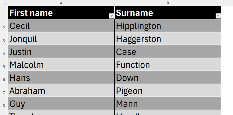
Excel is a great tool for presenting and analyzing information, but frustrations arise when the data isn’t appropriately laid out. Re-typing the data into the preferred layout takes time and is certain to result in errors. Luckily, there are ways to rearrange data in just a few simple steps.
There are many different ways to reorganize data in Excel, but we’ve listed some of the most useful and efficient methods.
Splitting Alternate Rows Into Two Columns
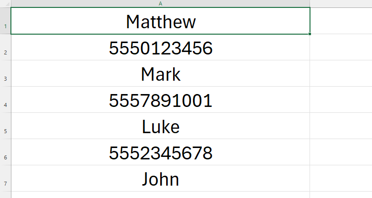
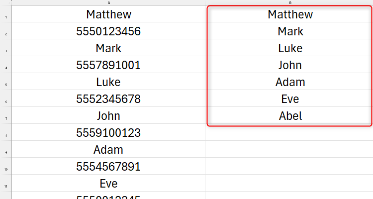
In this example, we have a spreadsheet containing people’s names and phone numbers in the cells below. You could end up in this situation if you’ve copied the data from another source (such as an email or a form) into your spreadsheet.
Excel is designed to display data in typical table form. In other words, each column should contain the same type of value (in our case, the person’s name in column A and the phone numbers in column B), and each row should contain details for one variable (in our case, each person).
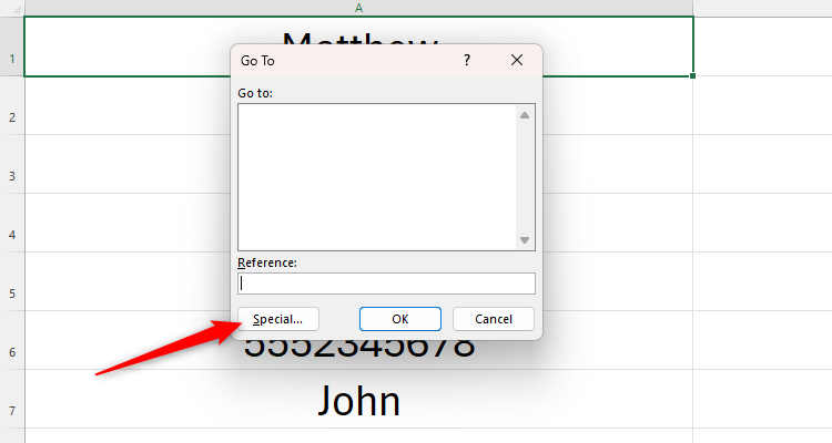
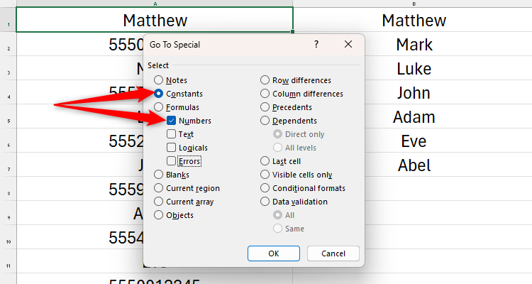
To achieve this, press Ctrl+G to launch the Go To dialog box. If you have other data in your sheet, first select the data you want to rearrange. Then, click “Special.”
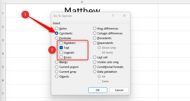
Then, choose the data type you want to select. In our case, we first want to select any cell that is constantly text (the people’s names), so we will click “Constants,” and then uncheck “Numbers,” “Logicals,” and “Errors,” leaving “Text” as the only checked data type.
Then click “OK.”
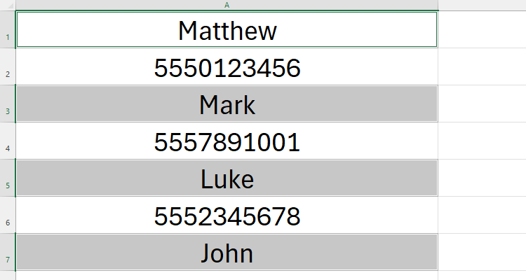
You will see that only the text is selected.
Then, press Ctrl+C to copy the text. Select the cell where you want to paste the first column of the new table you are creating, and press Ctrl+V. You’ll see that the data has handily pasted without gaps between each cell.
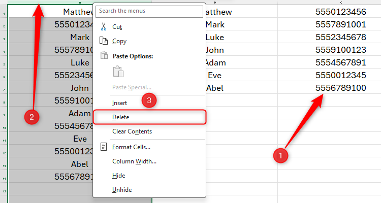
Repeat the process for the numbers, but this time, leave “Numbers” as the only checked constant data type.
Copy and paste the selected numbers into the column next to where you pasted the names, and then delete your original column by right-clicking the column header.
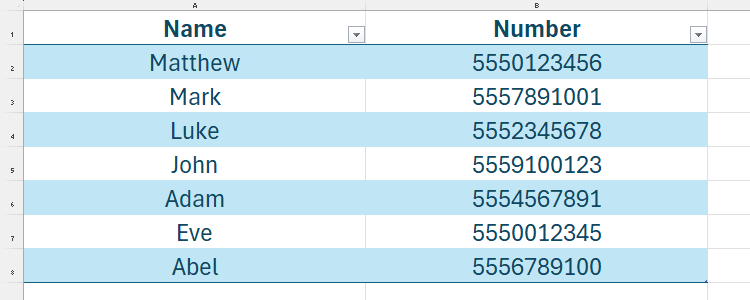
Using this method ensures the data remains in the same order, and you haven’t had to use any formulas in the process. You can also format your table to give you the option to sort the data or easily add further rows and columns.
As you saw when you opened the Go To Special dialog box, there are other types of data you can select and paste into a new column.
Turning Vertical Data Horizontal (Or Vice Versa)
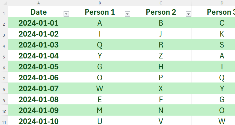
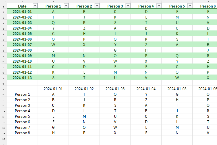
In the example below, we want to flip our table so that the dates run along the top and the people run down the side. Doing this manually would take a long time and inevitably lead to copying errors. Luckily, you can do this in just a few steps using Excel’s transpose pasting function.
Many online forums and tutorials state that you cannot transpose a formatted table, but this isn’t true. Indeed, the following process works regardless of whether or not your table is formatted using Excel’s Format As Table option.
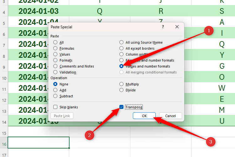
Select all the data in your table (including the header row), and press Ctrl+C. Then, click the cell where you want the top-left value of the transposed data to be, and press Ctrl+Alt+V to launch the Paste Special dialog box.
Now, you need to choose how the data will be converted. For example, because we have dates in our table, we want to make sure the number formats are correctly transposed. If we don’t pay attention to this, the dates will not transpose accurately. So, we have clicked the “Values and Number Formats” button. Then, check the “Transpose” checkbox, as this is the function that will switch your rows and columns for you. Finally, click “OK.”
You will then see the data transposed in the position you selected. You can now delete the original table and format the new one to suit your needs.
Sorting Data
Whether you want to sort numbers (ascending or descending) or text (alphabetically), there are various ways to achieve this. Which option you choose will depend on whether you’re sorting an isolated array (in other words, the column you’re sorting is not connected to any other data), or a column in a table.
Sorting an Isolated Array
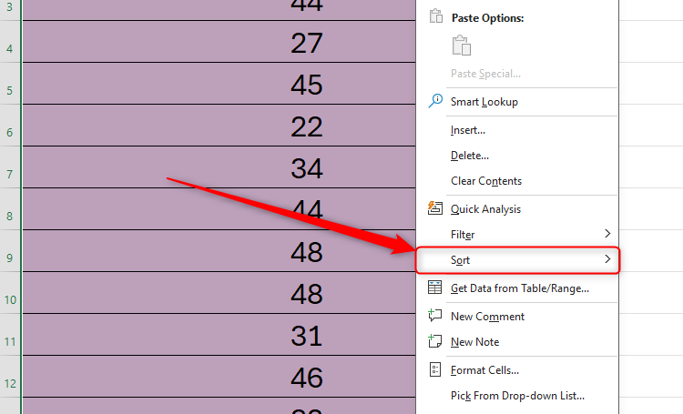
If you simply want to reorder an isolated array, select and right-click the data. In the menu that appears, hover over “Sort.”
You’ll then see several options. If your data is a series of numbers, you will have the option to sort them from smallest to largest or largest to smallest. Similarly, if you have a series of text, you can organize your data in alphabetical or reverse-alphabetical order.
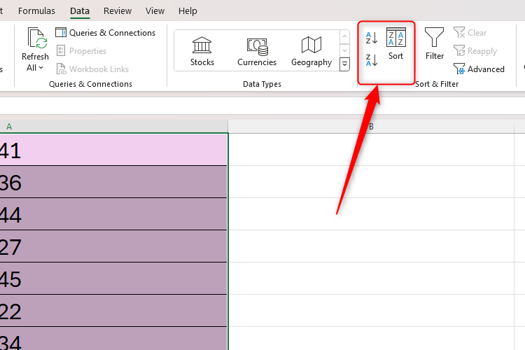
Alternatively, with your isolated array selected, see the options available in the Sort And Filter group of the Data tab on the ribbon. Here, you can either click the “A-Z” or “Z-A” buttons to rearrange your data quickly, or click “Sort” to launch more options.
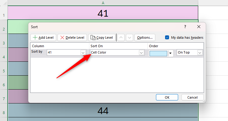
If you do click “Sort,” you will see the following dialog box. If you wish, you could sort the data based on cell or font color instead of the cells’ values.
Sorting a Column in a Table
If you use the above methods to sort a column in a table, the remaining columns will remain as they were, and your table will no longer read accurately. In this case, you need to add filter buttons to your table.
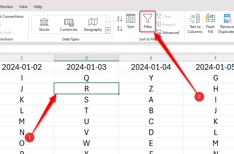
Select any cell within your table, and in the Data tab on the ribbon, click “Filter.”
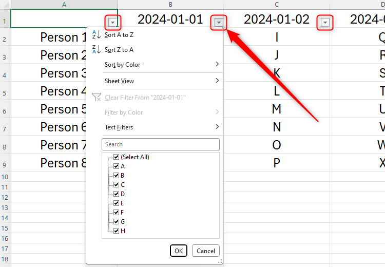
You will then see filter buttons, which you can click to rearrange a column with the knowledge that each row will remain congruent as you do this.
Formatting your data as a table using Excel’s Format As Table function will cause filter buttons to appear automatically.
Splitting and Merging Data Using FlashFill
There may be occasions when you want to split data into two or more cells—for example, if you have more than one piece of information in a cell, splitting this data into two cells means you’ll be able to use the sort function more effectively.
In this example, we want to split the names in column A so that the first names are in column B and the surnames are in column C.
Start by typing the first item in column B.
It’s important that you create the FlashFill column directly next to the existing data—otherwise, the FlashFill won’t work.
Then, select the cell directly underneath where you have typed the first entry, and press Ctrl+E. This will automatically follow the same pattern that you started in the first cell of this column, which, in our case, is extracting the first word from column A.
You can then repeat the process in column C for the surnames, as this is directly adjacent to existing patterned data.
To finish, format your table, delete the original data, and add filter buttons to make your data more flexible.
Follow the same process to merge data together. So, if you have data in columns A and B that you want to merge in column C, start by typing the first merged value in column C, and then press Ctrl+E to force Excel to follow the same pattern. You can also add further details when using FlashFill. For example, here, we have added the word “and” to the data.
It’s no good having nicely arranged data within your spreadsheets if your worksheet tabs are disorganized. Fortunately, Excel also lets you sort your tabs into alphabetical order.


