If you’re using Microsoft Excel on a Windows PC and enjoy using keyboard shortcuts to improve your productivity, you should definitely learn the many ways in which F4 can save you lots of time.
To follow along as you read this article, download a free copy of this Excel workbook. After you click the link, you’ll find the download button in the top-right corner of your screen.
Toggling Between Reference Types in Formulas
There are three types of references in Excel—relative references, absolute references, and mixed references—and you can use the F4 key to toggle between these when generating a formula.
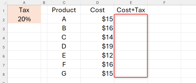
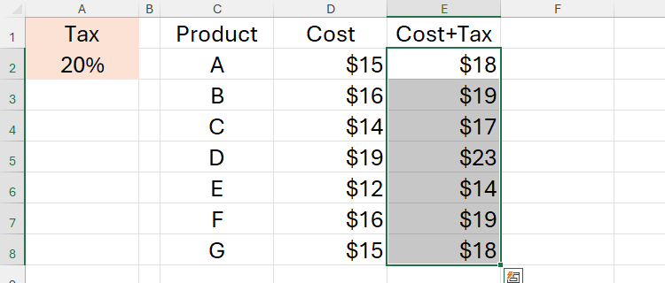
Let’s say you’re working out the cost of seven products in your store, and you need to add the mandatory 20% tax to those costs.
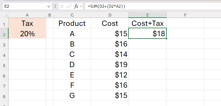
To do this, in cell E2, you might type:
=SUM(D2+(D2*A2))
and press Enter to add the 20% tax to the baseline cost.
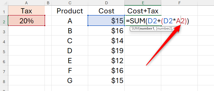
However, if you copy this formula to the remaining cells in column E, as you move down each row, the references in the formula will also move down a row—for example, the formula in cell E3 will reference cell A3, E4 will reference A4, and so on.
This is because, by default, Excel references are relative, meaning they use the same relative positioning between where you’re typing the formula and the cell they refer to if you copy the formula to a different location.

Related
How to Use Relative, Absolute, and Mixed References in Excel
Save time and reference the correct cells when creating formulas in Excel.
To fix this, you need to make the reference to cell A2 absolute using the F4 key. In other words, even when you copy the Cost+Tax formula to other cells in column D, you can use F4 to make sure the reference to cell A2 doesn’t change.
First, select cell E2, and press F2 to edit the formula. Then, use the Arrow keys to move the cursor directly before, in the center of, or directly after the cell reference you want to fix (in this case, it’s the reference to cell A2).
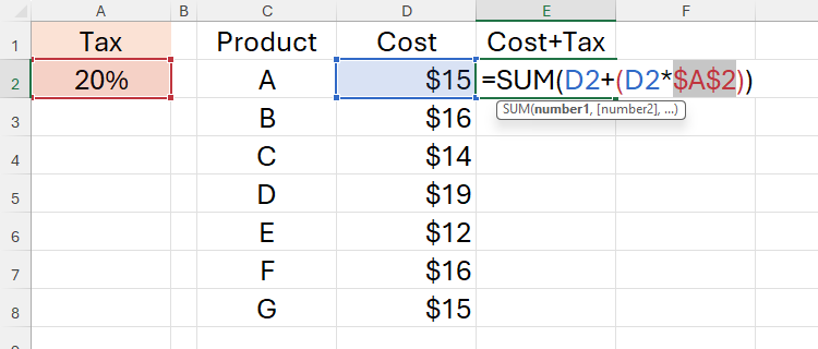
Now, press F4 once to toggle the reference type to an absolute reference. Instantly, you will notice a dollar sign ($) placed before the column and row references, turning “A2” into “$A$2.” This means that both the column and the row reference in this instance are locked, so when you copy the formula to other cells, the A2 reference will remain intact.
Depending on your keyboard setup, you might have to press the Fn key with F4 for it to perform the actions outlined in this guide. That said, if your keyboard has a function lock key, turn this on or off as appropriate to save you from having to press the Fn key every time.
After pressing Enter, you’re ready to duplicate the formula containing the absolute reference to the remaining rows. Press the Up Arrow key to head back to cell E2. Then, press Ctrl+Shift+End to select that cell and the remaining cells, then Ctrl+D to autofill the formula, safe in the knowledge that the reference to cell A2 will remain constant.
Next time, rather than pressing F4 after you have finished typing the formula, press it as soon as you type a cell reference in a formula to turn it into an absolute reference as you go.
The fun of using F4 to toggle between references doesn’t stop there. In this example, you need to work out how much your employees earn each year by adding their annual salaries to their fixed bonuses. In other words, you want to add the value in B2 to the value in D2 for the 2023 figure for employee A, and then you want to add the value in C2 to the value in D2 for their 2024 figure.
To create this calculation, you need the reference to the values in column D (the fixed bonus) to remain absolute, while references to the rows (each employee) and columns B and C (each year’s totals) need to be relative. This combination of absolute and relative references is called a mixed reference, and you can create this scenario using the F4 key.
To achieve this, in cell F2 type:
=SUM(B2+D2
Now, with your cursor still flashing after the reference to cell D2, press F4 three times so that only the column reference (D) has the dollar sign placed before it.
After closing the parentheses and pressing Enter, go back to cell F2, and press Ctrl+C to copy the formula. Then, press the Right Arrow to move to cell G2, and press Ctrl+V to paste the formula. Notice how the salary column reference switches relative to the cell position (B2 has changed to C2), while the fixed bonus column reference ($D2) remains the same.
Next, select cells F2 and G2 using Shift+Arrows, press Ctrl+Shift+End to also select the remaining cells, then press Ctrl+D to duplicate the formula, safe in the knowledge that the row references are relative, since they aren’t prefixed with the $ symbol.
When you toggled the reference types using F4 in the previous step, you will have noticed D$2 appearing as one of the options. If you used this mixed reference, the reference to the row would be absolute, while the reference to the column would be relative.
So, in summary, when typing a formula, you can press F4 repeatedly to cycle through absolute, mixed, and absolute references.

Related
The Best Excel Keyboard Shortcuts I Use as a Power User
The key to excelling in your spreadsheet work.
Repeating the Last Action
When you’re not typing a formula, F4 has a different use altogether that can save you a great deal of time.
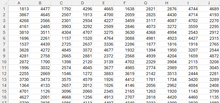
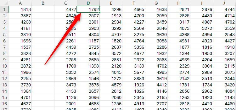
In this example, you’ve been asked to insert a blank column between each existing column of figures.
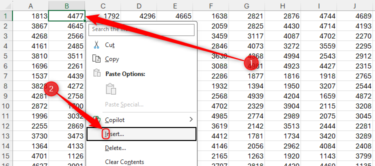
The first step to achieving this using only your keyboard is to move to cell B1, press the Menu key (also known as the Application key), then press i and Enter to open the Insert dialog box.
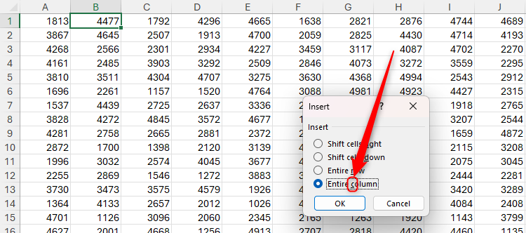
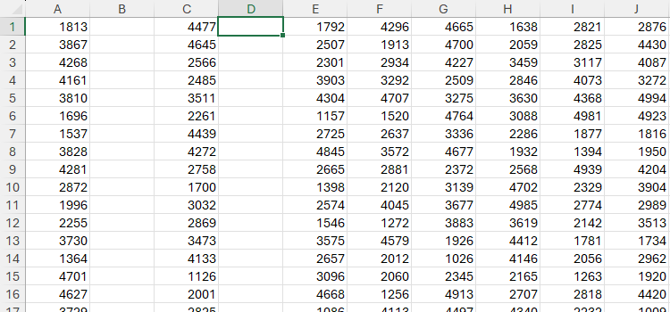
Next, press C and Enter to insert a new column to the left of column B.
Now that you’ve added an empty column between what were previously columns A and B, you could repeat this process for each new column, though the keyboard shortcut sequence is long-winded. This is where the power of F4 really comes in handy.
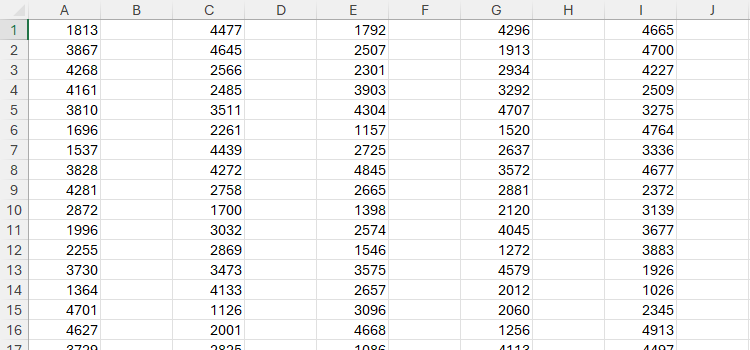
First, press the Right Arrow twice to move from cell B1 to cell D1.
Then, press F4 to repeat the last action you just performed (insert a new column to the left).
Then, use the same Right Arrow x 2 > F4 sequence to repeatedly and quickly add new columns between each existing column of data in your spreadsheet.
Next, let’s imagine you’ve been told that the blank columns you just added need to be 1 unit wide. To do this using your keyboard, first, use the Left Arrow to head back to cell B1. Then, press Alt > O > C > W > 1 > Enter to change the column width accordingly.
Again, this keyboard shortcut sequence is difficult to remember and perform quickly. However, since F4 lets you repeat the last action you performed, simply use the Right Arrow to head to column D, press F4, then move to column F, press F4, and so on. It took me less than five seconds to apply this column width change to the first 14 blank columns I created earlier.
You can use F4 to repeat various other previous actions in Excel, like changing a cell’s color or font formatting, adding or removing borders, or even duplicating the formatting of a shape or bars in a chart.

Related
Microsoft Excel Keyboard Shortcuts: Printable Cheat Sheet
Excel’s keyboard shortcuts are a real time-saver.
Performing and Repeating a Find Query
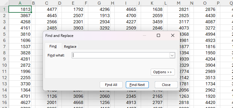
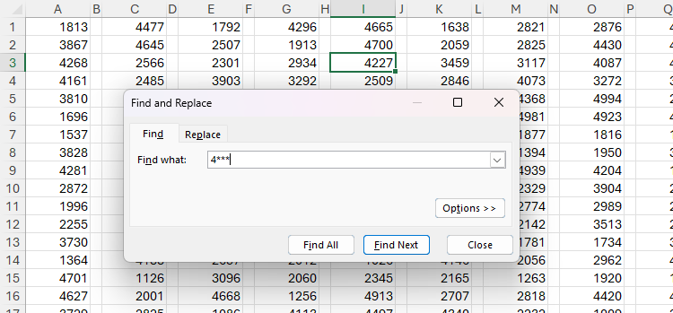
Many people know that pressing Ctrl+F opens the Find tab of the Find And Replace dialog box.

Related
How to Find and Replace Text and Numbers in Excel
The Find and Replace tool is a powerful and often forgotten feature of Excel.
Then, after typing the relevant search criteria in the Find What field, you can press Enter repeatedly to find each cell that matches those criteria.
The issue with this method is that if you want to make manual changes to your spreadsheet between each search result using only your keyboard, you have to press Esc to close the Find And Replace dialog box, make your changes, then press Ctrl+F to launch it again.
Instead, once you’ve typed the search query, press Esc to close the Find And Replace dialog box, and then press Shift+F4 to perform the search without relaunching the Find And Replace Dialog box. Each time you press Shift+F4 subsequently, the search continues as if the dialog box were still open, even if you make significant changes to the spreadsheets’ content.
The beauty of using this keyboard shortcut is that Excel remembers the last search query until you close the workbook.
Press Ctrl+Shift+F4 after closing the Find And Replace dialog box to move back to the previous search result.
Closing the Active Excel Workbook or Window
The final uses of the F4 key involve closing the Excel workbook or window.
When you press Ctrl+F4, the active workbook will either close (if you have AutoSave activated) or launch the Save As dialog box (if your workbook isn’t saved).

Related
How to Automatically Save Microsoft Excel Files to OneDrive
Yes, you can make Microsoft Excel automatically save your work.
Notice that while this closes the active workbook, the Excel window remains open, ready for you to open a new (Ctrl+N) or saved (Ctrl+O) worksheet. If you want to close the active Excel window altogether, press Alt+F4.
Using F4 and other keyboard shortcuts isn’t the only way to save time when working in Microsoft Excel. For example, you could personalize the Quick Access Toolbar so that your most-used features, like spell check, paste special, conditional formatting, and freeze panes, are accessible at a single click of your mouse.


