Quick Links
There are many ways to sort data in Microsoft Excel, and one of the simplest and most convenient is the SORTBY function. It lets you dynamically sort your data by more than one array while preserving the integrity of the original data.
At the time of writing (April 2025), the SORTBY function is only available to people using Excel or Office 2021 or later, Excel for Microsoft 365 on PC or Mac, Excel for the Web, or the Excel mobile and tablet apps.
The SORTBY Syntax
The syntax for the SORTBY function in Excel is both straightforward and logical:
=SORTBY(a,b¹,b²,c¹,c²...)
where
- a (required) is the range or array you want to sort,
- b¹ (required) is the first range or array by which you want the data to be sorted,
- b² (optional) is the sort order for b¹, and
- c¹ and c² (optional) are the second array and order by which you want to sort the data, and you can have up to 64 of these pairings overall.
If you omit the sort order arguments or type 1, the data will be arranged in ascending or alphabetical order by the specified range or array. On the other hand, type -1 to sort the data in descending or reverse-alphabetical order.
Arguments a, b¹, c¹, d¹, and so on must be compatible in terms of their dimensions. For example, if the range selected for argument a is 10 rows down, the arrays by which you want to sort the data must also be 10 rows down.
Using SORTBY to Sort By One Column
Let’s look at how the SORTBY function can be used to sort some data by one column.
To follow along as you read, download a free copy of the workbook used in this article’s screenshots. After you click the link, you’ll find the download button in the top-right corner of your screen.
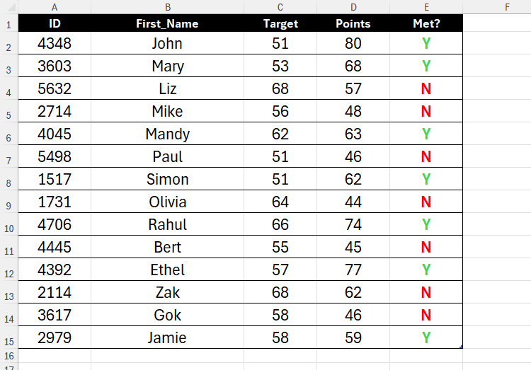
In this example, suppose you’ve been handed an Excel table named T_Targets, and you’ve been asked to sort the data by the Points column. At the same time, you need to leave the original table unchanged, as the information is structured in an order that must remain unaltered.
Related
The best way to do this is to use the SORTBY function.
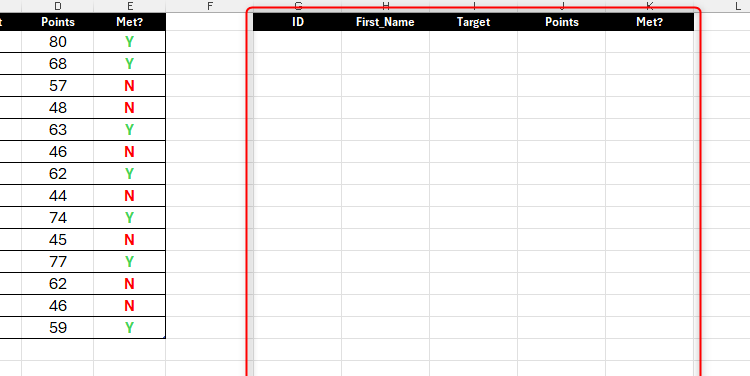
The first step is to prepare the area in your spreadsheet where the data will go. In this example, I’ve copied and pasted the column headers to cells G1 to K1, and I’ve adjusted the font size and alignment of cells G2 to K25 (to allow for vertical growth) to match the formatting of the original data.
Since the SORTBY function returns a dynamic array, make sure there are enough vacant cells to display the result in full. Otherwise, you’ll get the dreaded #SPILL! error when you complete your formula.
Next, in cell G2, type:
=SORTBY(T_Targets,T_Targets[Points],-1)
where
- T_Targets is the array,
- T_Targets[Points] is the name of the column containing the data that the array will be sorted by, and
- -1 tells Excel to sort T_Targets[Points] in descending order.
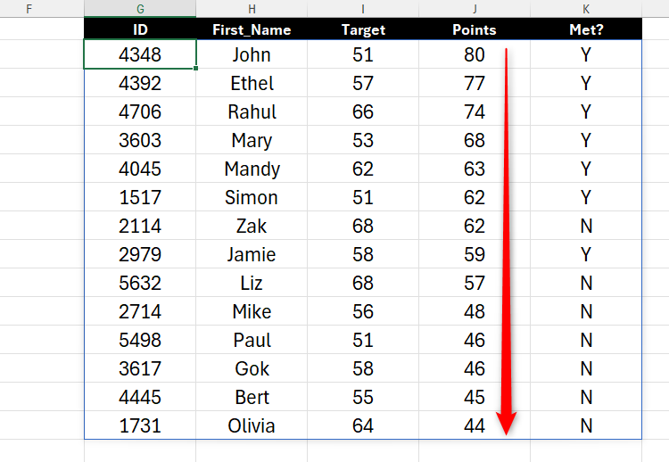
When you press Enter, you’ll see the result reorder your data by the Points column. A blue line around the result reminds you that it’s a dynamic array (in other words, the result has spilled from cell G2 to the other cells).
The SORTBY formula doesn’t have to be in the same worksheet—or even the same workbook!—as the source data. However, if you use SORTBY between workbooks, both files must be open—otherwise, you’ll get a #REF! error.
You can then apply conditional formatting to the result to aid further analysis. For example, you might want to color the rows of people who have met their target green, and those who haven’t red.
Using SORTBY to Sort By More Than One Column
One benefit of using SORTBY instead of SORT in Excel is that you can choose more than one variable by which to sort your data.
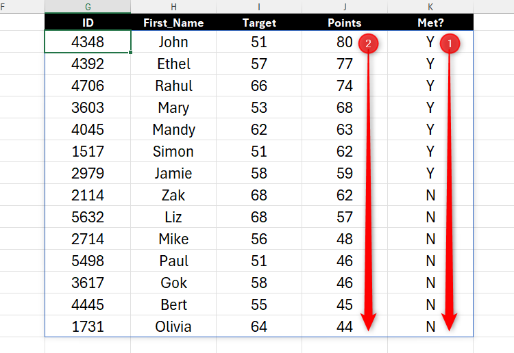
Staying with the same example as above, let’s now assume that while you still want to sort the individuals by their points total, you want everyone who has met their target to be above those who haven’t in the table. In other words, you want to sort the data by the Met? column, and then by the Points column.
After preparing the cells where the data will go, including duplicating the column headers and deleting any previous SORTBY function you typed, in cell G2, type:
=SORTBY(T_Targets,T_Targets[Met?],-1,T_Targets[Points],-1)
where
- T_Targets is the array,
- T_Targets[Met?] is the first sort-by column in that array,
- -1 tells Excel to sort T_Targets[Met?] in reverse-alphabetical order (the Ys above the Ns),
- T_Targets[Points] is the second sort-by column, and
- -1 tells Excel to sort T_Targets[Points] in descending order.
Here’s the result you’ll get when you press Enter. Notice how the points totals for people who have met their target are grouped together and displayed in descending order, and the same goes for those who haven’t met their target.
Using SORTBY With FILTER
The SORTBY function can be used with other functions in Excel to further refine the result. Specifically, I’ll show you how to use SORTBY with FILTER to sort and filter the data in a new array at the same time.
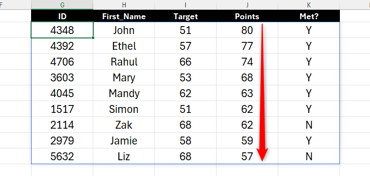
Let’s say your aim now is to produce a result that sorts the data by the Points column, but only shows people who scored more than 55 points overall.
After creating column headers for the result in row 1, in cell G2, type:
=FILTER(SORTBY(T_Targets,T_Targets[Points],-1),SORTBY(T_Targets[Points],T_Targets[Points],-1)>55)
and press Enter.
Let’s break this formula down to explore in more detail how it works.

Related
The FILTER function requires two arguments: the array and what to include in the filter. So, the part of the formula that reads:
SORTBY(T_Targets,T_Targets[Points],-1)
is the FILTER function’s array argument. However, by nesting SORTBY in this argument, you’re telling Excel that the array is the table named T_Targets, but with the data sorted by the Points column in descending order.
Then, the part that reads:
SORTBY(T_Targets[Points],T_Targets[Points],-1)>55
is the FILTER function’s inclusion criteria. However, because the array argument uses sorted data, you need the inclusion criteria to be sorted as well. In this case, the array containing the data to sort is the Points column, and the same column is the array you used earlier to sort the data in descending order. Then, the final part of the inclusion criteria tells Excel to only include values in this sorted array that are greater than 55.
SORT vs. SORTBY in Excel
While the SORT and SORTBY functions are both intended to reorganize data based on certain values in the data, they work in slightly different ways:
|
Characteristics |
SORT Function |
SORTBY Function |
|---|---|---|
|
Formula syntaxes |
The SORT function lets you define the array, a column index number to sort by, the sort order, and the option to sort by a row instead of a column. |
The SORTBY function lets you define the range, and up to 64 sort array-order pairings. |
|
Sorting levels |
When using the SORT function, you can only sort by one row or column. |
When using the SORTBY function, you can sort by up to 64 rows or columns. |
|
Argument references |
The row or column to sort by is referenced by an index number, meaning if you add or remove rows or columns in the original data, this index number may become outdated. |
Since the array or arrays to sort by can be a named reference—like column headers—this reference will remain constant, even if you add or remove columns in the original data. |
Another way to create a new version of a dataset that you can manipulate—all while leaving the original data intact—is to create a PivotTable. This powerful Excel tool lets you summarize and reorganize your data in various ways, meaning you can quickly generate calculations and analyze your figures without using complex formulas.


