

While Microsoft Excel offers many tools for formatting data in various ways, sometimes, the built-in tools don’t quite do exactly what I’m looking for, or take up too much time to execute. In these scenarios, I use custom number formatting to quickly create a number format that meets my needs.
Disclaimer: There are some scenarios where using conditional formatting is preferable over using custom number formatting, such as coloring whole rows based on a value. However, in situations where I could use either to generate the same or similar outcomes, I opt for the latter. In this article, I’ll explain why.
What Is Custom Number Formatting, and How Does It Work?
In Excel, every cell has its own number format, which you can review by selecting a cell and looking at the Number group in the Home tab on the ribbon.


Related
Excel’s 12 Number Format Options and How They Affect Your Data
Adjust your cells’ number formats to match their data type.
One of the number format options you can apply to a cell is a custom number format, which you can access by clicking the Number Format dialog box launcher, before clicking “Custom” in the Format Cells dialog box.
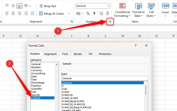
If you prefer using Excel keyboard shortcuts, press Ctrl+1 to launch the Format Cells dialog box, press Tab to activate the Category menu, and type Cus to jump to Custom.
By the end of this guide, you’ll be able to use custom number formatting to create spreadsheets that look something like this:

If you’ve never used custom formatting before, it might seem confusing at first, and I can see why you might think that using conditional formatting instead would be the better option. However, Excel processes custom number formatting much more quickly than conditional formatting, and—once you understand its logic—you’ll likely find it quicker and easier to use.
Personally, one of the main reasons I prefer using custom number formatting is that everything happens in one place—there’s no need to jump back and forth between different dialog boxes to add various rules, so the process is time-saving and straightforward.

Related
Short On Time? Use These Excel Tips to Speed Up Your Work
Use Excel’s time-saving tools to get jobs done.
Before I go ahead and guide you through some examples, let me explain how custom number formatting works.
Custom number formats are entered in the Type field in the Custom section of the Format Cells dialog box.

The code you need to insert here follows a strict order:
POSITIVE;NEGATIVE;ZERO;TEXT
In other words, the first argument in the custom number format field dictates how positive numbers are formatted, the second argument dictates how negative numbers are formatted, the third argument dictates how neutral numbers are formatted, and the fourth argument dictates how text is formatted. Notice, also, how semicolons are used to separate each argument.
For example, typing:
#.00;(#.00);-;"TXT"
into the Type field displays:
- A number with two decimal places for positive numbers (#.00),
- A number with two decimal places in parentheses for negative numbers (#.00),
- A dash for zeros (-),
- And the letter string “TXT” for all text values (“TXT”).

If you leave out any of the arguments by adding the semicolon but not typing any code, the relevant cells in your spreadsheet will appear blank.
For example, typing:
#.00;;;"TXT"
into the Type field displays a number with two decimal places for positive numbers, produces a blank cell for negative numbers and zeros, and displays “TXT” for all text values.

Even though the values displayed in each cell depend on what you specify in the custom number format Type field, the actual values of the cells remain unchanged. In the example above, even though cell C2 appears blank (because I omitted the NEGATIVE argument in the Type field), when I select the cell, the formula bar reveals its true value.

This means that I could still use this cell in formulas if required.
Related
The Beginner’s Guide to Excel’s Formulas and Functions
Everything you need to know about Excel’s engine room.
As well as using custom number formatting to change what value appears in a cell, you can also change the color of the values and add symbols to visualize your data. Let’s look into this in more detail.
Changing the Font Color Using Custom Number Formatting
Microsoft Excel’s custom number format lets you define the color of the values in the selected cells. What’s more, for the main eight colors (black, white, red, green, blue, yellow, magenta, and cyan), you don’t need to remember any code—you can simply type the color name. Colors must be the first argument for each data type, and they must be placed in square parentheses.
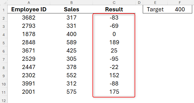
Let’s take this example, which shows whether ten employees have met their sales targets. You want all the positive numbers in column C to be green, negative numbers red, and zeros blue.
To do this, select cell C2, open the “Format Cells” dialog box (Ctrl+1), and head to the “Custom” section.
In the Type field, enter:
[Green]#;[Red]#;[Blue]0;
to tell Excel to keep positive and negative numbers as they are (#)—but formatted green and red, respectively—and zeros as “0”—but formatted blue. Since there’s no text in this range, you don’t need to specify a number format for text values, so only the first three arguments are required.
When you click “OK,” you’ll see the text change color accordingly. You can then click and drag the fill handle to the final row of data to apply this custom number format to the remaining values. This won’t change the values in column C, since they’ve been calculated using a formula.

If you want to use colors other than the standard eight on offer for the font, instead of typing the color name in square parentheses, type the color code:
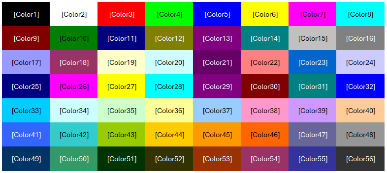
For example, typing:
[Color10]#;[Color30]#;[Color16]0;
would use a dark green font for positive numbers, a crimson font for negative numbers, and a gray font for zeros.
To revert the number formatting back to its original, select the cells containing the formatted data, and in the Number group of the Home tab on the ribbon, select “General” in the drop-down list.
At this point, take a moment to appreciate how achieving the same outcome using conditional formatting would require you to create three separate rules. On the other hand, using custom formatting, you can make these changes by adding a few characters to the Type field.
Displaying a Symbol Using Custom Number Formatting
Much like when using conditional formatting, you can display symbols according to the corresponding values through custom number formatting.
Using the same example as above, let’s say you now want to convert the numbers in the Result column (column C) to up arrows for positive numbers, down arrows for negative numbers, and an equal (=) sign for zeros.
To do this, you first need to locate the symbols, or know their keyboard shortcuts.
In the Insert tab, click “Symbol,” and insert the symbols in another area of the spreadsheet, so you can copy and paste them into your custom code.

Alternatively, use the Windows shortcut Windows+Period (.) to launch the emoji keyboard, and insert these straight into the Type field.
On the other hand, I know that the Windows keyboard shortcut for ▲ is Alt+30, and ▼ is Alt+31, and I can use these shortcuts when typing in the Type field.
So, select cell C2, and in the Custom section of the Format Dialog box (Ctrl+1 > Tab > Cus), type this very short line of code:
▲;▼;"=";
to tell Excel to replace positive numbers with “▲,” negative numbers with “▼,” and zeros with “=.”
Any text strings or typed symbols (including mathematical or any keyboard symbols) must be placed in double quotes.
Now, press Enter, and use the fill handle to apply the custom number formatting to the remaining cells in the column.
Next, you might want to color the arrows to visualize your data more clearly. This is where you combine the color code with the arrow symbols, remembering that the color code must always be placed at the start of the argument.
To do this, type:
[Green]▲;[Red]▼;"=";
into the Type field. Here’s what you’ll see:
Using Custom Number Formatting for Font Colors, Numbers, and Symbols
Now, it’s time to combine all the steps above to produce an outcome that shows colored symbols and arrows at the same time.
In the Type field for cell C2, type:
[Green]#▲;[Red]#▼;0" =";
where:
- The first argument ([Green]#▲) turns positive values green, displaying both the number and an upward triangle,
- The second argument ([Red]#▼) turns negative values red, displaying both the number and a downward triangle, and
- The third argument (0″ =”) doesn’t have any color formatting (so adopts the manual cell formatting), and displays the number “0” followed by a space and the “=” sign.

To align the number to the left of the cell, and the symbol to the right of the cell, type an asterisk (*) and a space between the symbol and number in each argument (for example, [Green]#* ▲;[Red]#* ▼;0* ” =”;). The asterisk tells Excel to repeat the following character infinitely (until the cell’s boundary is met), and since the following character is a space, the gap between the number and the symbol increases and decreases with the cell width.
In a final example, let’s say you’ve worked out the percentage change in points totals for various sports teams, and you want to quickly format the positive and negative figures so that they turn green or red, have an up or down arrow, include the number, and are considered percentages. You also want zeros to display as dashes.

To do this, in the Type field for the cells in column C, type:
[Green]▲#%;[Red]▼#%;"-"
Here’s what you’ll get for the result:
Once you’ve practiced using custom number formats to add color and symbols to your cells, you’ll realize how quick and easy the process is—and, hopefully, you’ll use custom number formatting more often in the future!


