Mastering Microsoft Excel’s tools is a never-ending process, even for those who have used the program at work or at home for decades. With this in mind, here are some of my favorite Excel hacks I’ve picked up over the years that you can take away and use to speed up your spreadsheet workflow.
1
You Don’t Need to Freeze the First Row of a Table
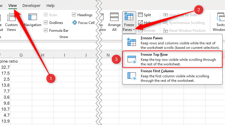
If you’re working with an Excel sheet containing lots of rows of data, you might be tempted to freeze the first row via the View tab on the ribbon, so that when you scroll down, the headers remain visible.
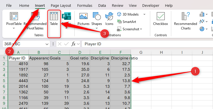
However, you don’t need to take this step if you format your data as an Excel table. To do this, first, make sure your data has column headers in the top row. Then, select your data, and in the Insert tab on the ribbon, click “Table.”
If you have lots of rows of data, rather than selecting them manually with your mouse, activate the top-left cell (in my case, cell A1), press Ctrl+Shift+Right to select the whole row, and then press Ctrl+Shift+Down until all your data is selected.
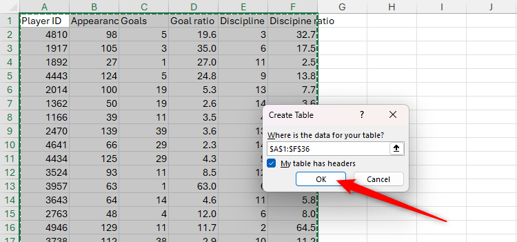
Now, ensure the information in the Create Table dialog box is correct, and click “OK.”
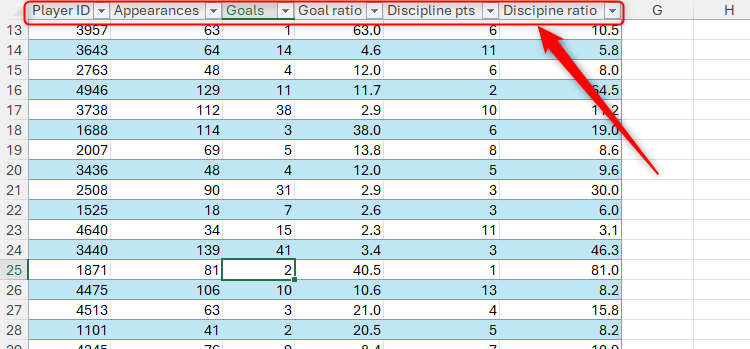
Finally, select any cell in the table, and scroll down. Notice that the column headers (A, B, C, and so on) are replaced by the column names you assigned at the start.
This trick only works if your table contains more rows than can fit on your screen. Otherwise, the table headers are always on show, so there’s no need for the spreadsheet headers to repeat those labels.
2
Copy and Access Multiple Items at the Same Time
Most people know about the famous keyboard shortcuts for copying (Ctrl+C) and pasting (Ctrl+V) items in Excel. However, fewer people know that you can copy several items from various sources at the same time, and paste them into a spreadsheet with a single click.
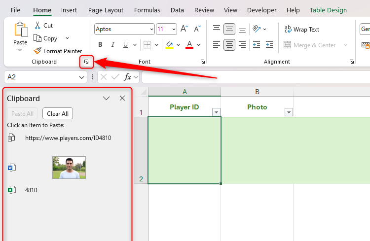
Let’s say you’re creating a player profile spreadsheet for your favorite soccer team. For each player, you want their ID, a photograph, and a link to their online bio.
Even though the player IDs are on a separate worksheet, their photographs are in a Microsoft Word document, and their online bio URLs are accessed in a web browser, you can go ahead and copy each item one by one.
Then, head back to the spreadsheet where you want the copied items to go, and click the Clipboard launcher icon in the Home tab on the ribbon to see the items you just copied in the Clipboard pane. Notice, also, how each item has an icon next to it to remind you of its original location.

Related
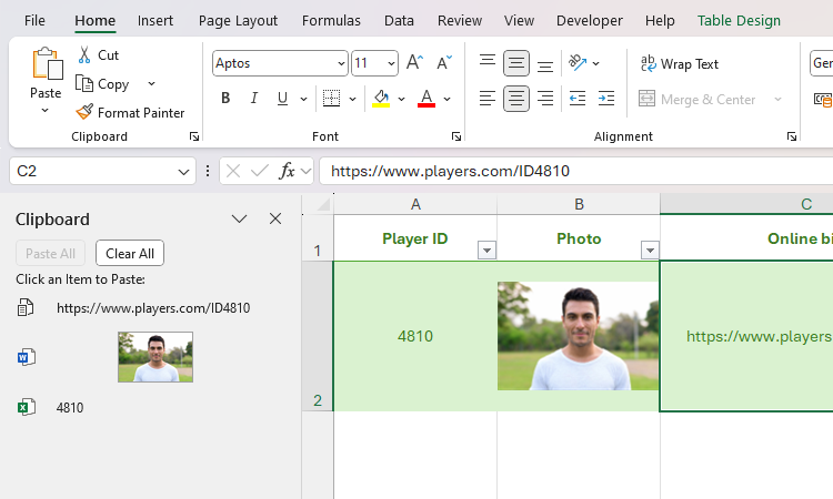
Now, select the cell where you want the first item to be pasted, and click the item in the Clipboard pane. Repeat this process for the other items you copied.
After pasting a picture in Microsoft Excel, right-click it and select “Place In Cell” to embed the image within the boundaries of the cell.
You can then click “Clear All” in the Clipboard pane, before moving on to the next batch of items you want to copy and paste.
The Microsoft Excel clipboard can hold up to 24 items. This means that when you copy a 25th item, it will replace the oldest item on the clipboard.
The benefit of using the Microsoft Excel clipboard, rather than the Windows clipboard (Windows+V), is that it remains on show in the Excel window until you close it manually. On the other hand, the Windows clipboard disappears as soon as you click away from it.
3
View All Formulas Used in Your Spreadsheet
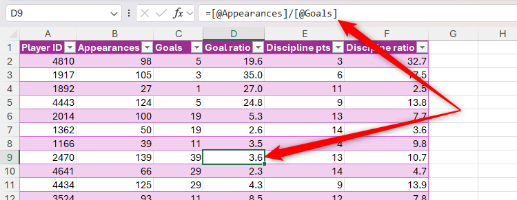
By default in Excel, worksheet cells display formula results, while the formula bar shows the formula you used to get that result.

Related
The Beginner’s Guide to Excel’s Formulas and Functions
Everything you need to know about Excel’s engine room.
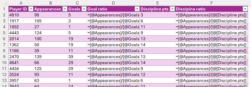
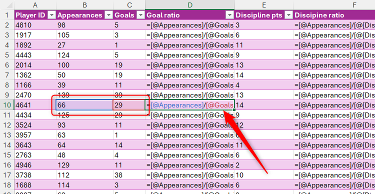
However, you can also display the formulas in the cells themselves. To do this, press Ctrl+` (the grave accent key, which is usually in the upper-left corner of the keyboard).
When you use this keyboard shortcut, you can quickly see which cells contain formulas, understand how the calculations are made, and check for any errors. What’s more, with this option activated, selecting a cell containing a formula will color the cells it references, making troubleshooting more straightforward.
Press Ctrl+` again to return your spreadsheet to the default state.
4
See All Worksheets Tabs With a Right-Click
One of the more frustrating tasks in Excel is navigating the tab manager at the bottom of the screen, especially if you have many worksheets within your workbook. Indeed, clicking the tiny arrows in the bottom-left corner of the Excel window to scroll through the tabs takes up too much of your precious time.
Click and drag the three dots next to the right of the worksheet tabs to create more space for their names.
One way to speed up this process is to press Ctrl+Page Down to move to the next tab, or Ctrl+Page Up to jump back to the previous tab.
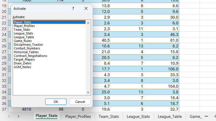
However, my preferred method is to right-click the tab navigation arrows. Doing this launches the Activate window, and you can then double-click the sheet you want to navigate to (or use the arrow keys and press Enter).
This tool is particularly useful if you’ve taken the time to give your worksheets short but descriptive names, rather than sticking with the default Sheet1, Sheet2, Sheet3, and so on.
5
Use the Status Bar for Quick Calculations
One of the simplest yet probably most under-used tools in Excel is the Status Bar, which sits in the bottom-right corner of the Excel window.
Related
How to Customize and Use the Status Bar in Excel
The status bar at the bottom of Excel’s window can tell you all kinds of interesting information.
Specifically, when you select some data in your spreadsheet, the Status Bar provides calculations for instant analysis without requiring additional formulas.
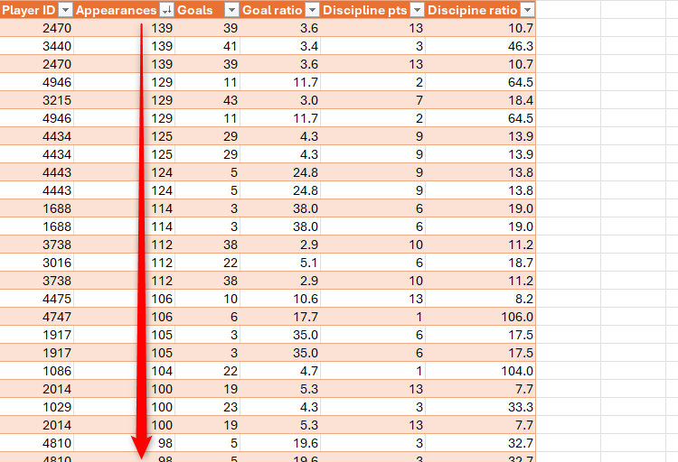
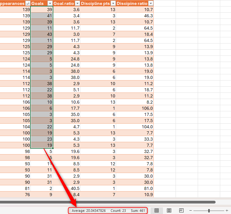
In this example, the table is sorted by appearances in descending order, and I quickly want to see the total and average goals scored by anyone who has played 100 or more games.
While I could use formulas to generate this information, I don’t want the result to appear in the spreadsheet—my aim here is just to take a glance at the figures for a quick analysis.
So, as soon as I select the goal totals for the relevant players, the average, count, and sum of the selected cells appear in the Status Bar.
If you can’t see these totals in your version of Excel after you select two or more cells containing data, right-click the Status Bar, and check the aggregation calculations you want to display from the six options—Average, Count, Numerical Count, Minimum, Maximum, and Sum.
What’s more, I can click any of these calculations in the Status Bar to copy the values to my clipboard, ready to be pasted elsewhere as necessary.
If you’re keen to save time when using Microsoft Excel, as well as using the hacks I’ve shared with you in this guide, make the most of the name box to speed up navigation, and personalize the Quick Access Toolbar to perform your most-used commands in an instant.


