Despite having worked in Microsoft Excel for decades, I’m always learning new ways to speed up my workflow. Specifically, I’ve stumbled upon some keyboard shortcuts over the past couple of years that I now use every day, and I wish I’d known about them sooner!
1
F2: Enter a Cell’s Edit Mode
When you enter a formula into Excel and press Enter, the cell displays the result, and the formula bar displays how you got there. In this example, cell C1 shows the result of a SUM formula that adds the value in cell A1 to the value in cell B1, while the formula bar reveals the formula itself.

Related
Lied On Your Resume About Excel Expertise? 8 Concepts You Need to Learn Right Now
A whistle-stop tour of Microsoft Excel’s must-knows.
Let’s suppose you later realize that you actually needed to multiply the values in cells A1 and B1 rather than add them together. To do this, you could edit the formula in the formula bar, or double-click cell C1 and amend the formula there. However, both of these methods (which I previously believed were the only methods!) require you to use your mouse, thus disrupting your workflow and requiring you to move away from your keyboard.
Instead, use the Arrow keys to navigate to the cell you want to edit, and press F2. This activates the edit mode for that cell, meaning you can use the Arrow keys again to move along the formula, and make the required changes using only your keyboard.
When you’ve finished making the necessary changes, press Ctrl+Enter to finalize the result and keep that cell active, so that you can double-check the formula in the formula bar.
2
Ctrl+Shift+V: Paste Values Only
If you use Ctrl+V when pasting data from another source—like a web page, Word document, email, or another workbook or worksheet—into Excel, as well as pasting the values, the program adopts the source formatting, including any background colors, text colors, fonts, bold, italics, and so on.
In this example, when I pasted the first five rows of a table from a Wikipedia page using Ctrl+V, the cells were formatted inconsistently, the national flags covered the country names, and some of the text was hyperlinked. As a result, I had to take extra steps to remove this formatting and tidy up the data.
Instead, Excel lets you paste the copied content into your worksheet while preserving the destination formatting. There are various old-school ways to do this, such as clicking the “Paste” drop-down menu in the Home tab on the ribbon and selecting “Values,” or using the original keyboard shortcut, Ctrl+Alt+V > V.
However, in 2022, Microsoft introduced a simpler keyboard shortcut to paste the values only: Ctrl+Shift+V. Notice how using this shortcut pastes the Wikipedia data as unformatted values without the national flags.
As a result, I only need to make one or two small changes to tidy up the data.
Also, I can select any cell in the data and press Ctrl+T to convert the details into a formatted Excel table.
Related
Everything You Need to Know About Excel Tables (And Why You Should Always Use Them)
This could totally change how you work in Excel.
As well as copying data from a website and pasting it into Excel, you can also import online tables using the Data tab on the ribbon.
3
Ctrl+Shift+L: Filter Columns
Filters are an invaluable tool in Excel to display only the rows that meet certain criteria you set, making data scouring and analysis much more straightforward.
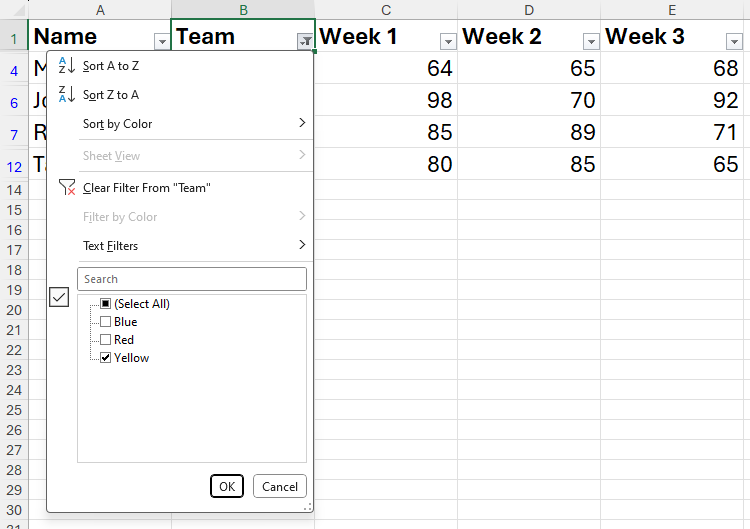
Whether you’re working with data formatted as a table or a series of contiguous data in unformatted cells, select any cell in the range, and press Ctrl+Shift+L to add filter buttons to the first row of the data.
Then, press Ctrl+Up to jump to the header row containing the filters, use the Left and Right Arrow keys to navigate to the column you want to filter, and press Alt+Down to launch the filtering options.
To reset all the filters, select any cell in the range, and press Ctrl+Shift+L twice. The first press removes the filter buttons and, thus, any filters applied, and the second press re-adds the filter buttons to the first row of your data.

Related
How to Sort and Filter Data in Excel
Microsoft Excel has power sorting and filtering options. Here’s how to use them in your spreadsheet.
4
F4: A Versatile Keyboard Shortcut
Probably my favorite and most used Microsoft Excel keyboard shortcut is the impressively versatile F4.
Toggling Between Reference Types in Formulas
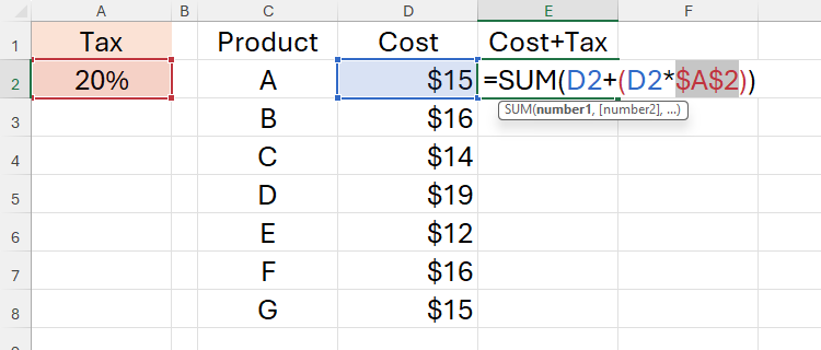
First, F4 lets you toggle between relative, absolute, and mixed references in a formula to fix or unfix references to certain cells, columns, or rows. In this example, I pressed F4 after typing the reference to cell A2 in my formula to add the dollar symbols ($), forcing Excel to fix this reference when I eventually copy the formula to other cells.

Related
How to Use Relative, Absolute, and Mixed References in Excel
Save time and reference the correct cells when creating formulas in Excel.
Repeating the Previous Action
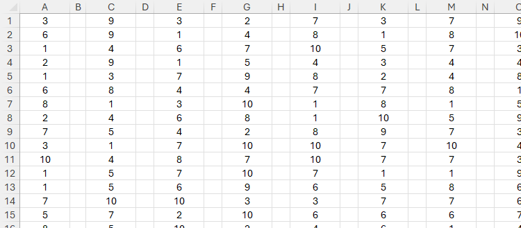
Second, you can use F4 to repeat the last action you performed on your worksheet. In the screenshot below, after manually reducing the width of column B by clicking and dragging the right side of the column header to the left, I selected cell D1 and pressed F4, and repeated this process for the other blank columns to make sure they were all resized consistently.
You can use F4 to repeat any action in Excel, like pasting data, formatting a cell, deleting rows or columns, and many more.
Repeating a Search
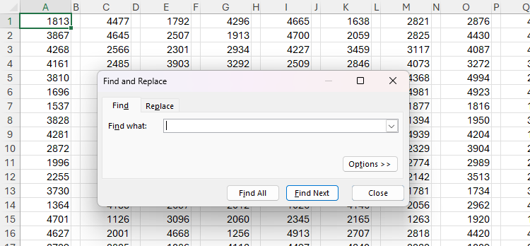
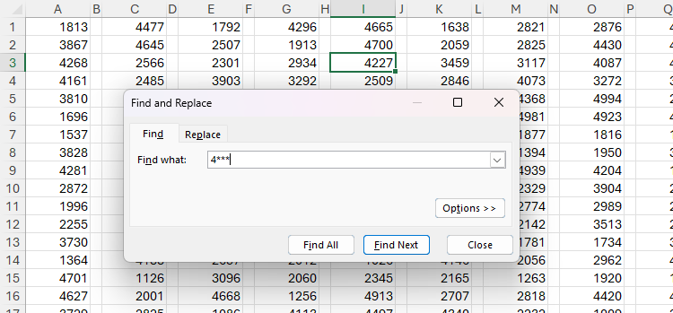
Third, Shift+F4 lets you repeat the last search you performed. Start by pressing Ctrl+F to open the Find tab of the Find and Replace dialog box.
Then, after typing the relevant search criteria in the Find What field, you can press Enter repeatedly to find each cell that matches those criteria.
However, if you need to make manual changes to your spreadsheet between each result using only your keyboard, you’ll need to press Esc to close the dialog box, make your changes, and then press Ctrl+F to launch it again.
Instead, once you’ve typed the search query, press Esc to close the dialog box, then press Shift+F4 to repeat the search to find the next cell that meets the criteria. Each time you press Shift+F4 thereafter, the search continues as if the dialog box were still open, even if you make significant changes to your spreadsheet. Alternatively, press Ctrl+Shift+F4 to move back to the previous search result.
Closing the Excel Workbook or Window
A fourth and final use of F4 comes in handy at the end of the workday, when you’re ready to switch off and go home:
- Ctrl+F4 closes the active workbook, but leaves the Excel window open. If the workbook isn’t saved, you’ll see the Save As dialog box first.
- Alt+F4 closes the active Excel window altogether.
5
Ctrl+1: Format Cells
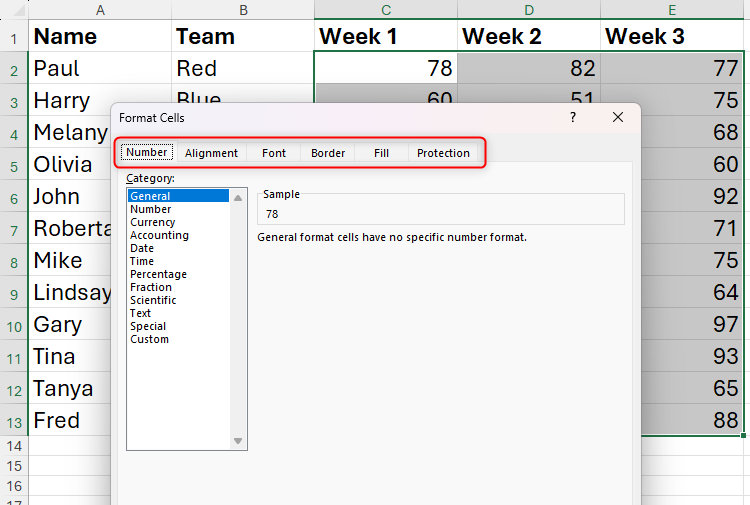
Ctrl+1 in Microsoft Excel launches the Format Cells dialog box, which is where you can change the number format, alignment, font, border, fill, and protection properties of a single cell or range of cells.
The alternative routes to the same outcome are to right-click a cell and select “Format Cells,” or search the ribbon for the formatting tool you want to apply—both of which take significantly more time than this easy-to-remember keyboard shortcut.
After selecting the cell or cells you want to format and pressing Ctrl+1, use the Left and Right Arrow keys to jump between the tabs in the Format Cells dialog box.

Related
Excel’s 12 Number Format Options and How They Affect Your Data
Adjust your cells’ number formats to match their data type.
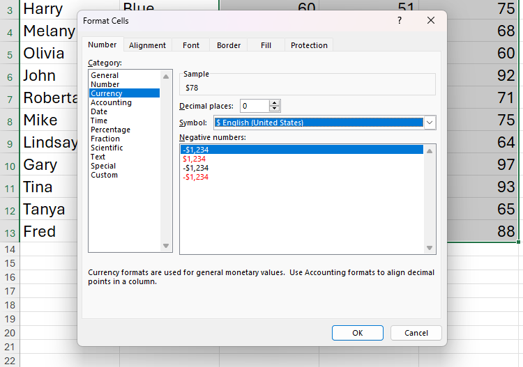
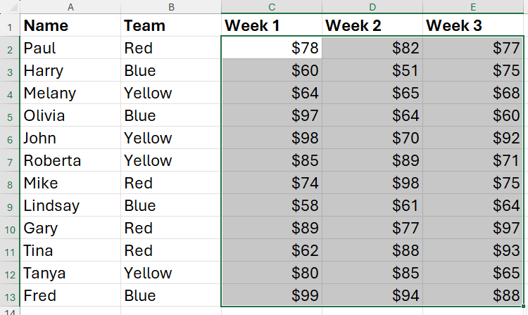
Then, once you’ve landed on the relevant tab, press Tab to jump between the options. In this case, I want to format the selected cells so that their values are currencies, so after navigating to the Number tab and pressing Tab, I’ll use the Down Arrow key to select “Currency.” Then, I’ll press Tab again to navigate through and adjust the currency options.
Then, once I’ve selected all the relevant formatting for those cells, I can press Enter to save the changes and close the dialog box.
6
Spacebar: Check and Uncheck Checkboxes
The final keyboard shortcut that I couldn’t live without today—having discovered it just over a year ago—is the Spacebar.
You might have come to this article looking for groundbreaking keyboard shortcuts you’ve never seen before—but bear with me: the Spacebar is a real time-saver for anyone using checkboxes in their spreadsheet.
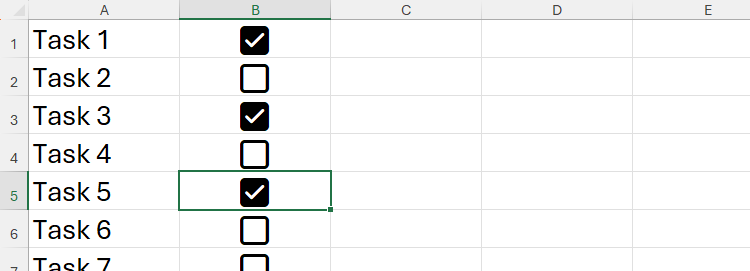
Rather than using your mouse to laboriously check and uncheck checkboxes in Excel, use the Arrow keys to navigate a cell containing a checkbox, and press Spacebar to add or remove the checkmark.
Likewise, if you select several cells containing a checkbox (using Shift+Arrow keys) and press the Spacebar, they’ll all be checked and unchecked at the same time.
To delete a checkbox from your worksheet, select the cell where the checkbox is located, and press Delete. If your checkbox is checked, pressing Delete will first uncheck the checkbox, and pressing it again will remove it altogether.
The shortcuts I’ve discussed in this guide are just a few of the many Microsoft Excel keyboard shortcuts you can learn to complete your work more quickly and move one step closer to being a power user. You can also download, print, and pin our printable cheat sheet to your notice board, so that you can access them whenever you need to!


