Don’t Use MATCH in Microsoft Excel: Use XMATCH Instead

There are many ways to extract values from data in Microsoft Excel, and two such examples are the MATCH and XMATCH functions. However, since Microsoft introduced XMATCH to Excel in 2021, I’ve ditched MATCH altogether, and in this guide, I’ll explain why you should too.

Microsoft Office 2024

Gain permanent access to Word, Excel, PowerPoint, and OneNote with the Office Home 2024 bundle. It isn’t a one-to-one replacement for a Microsoft 365 subscription, as it lacks some apps and does not include feature updates, but it’s a one-time purchase, so it’s ideal for those who just need the basics.

The MATCH Function in Excel

Microsoft Excel’s MATCH function tells you the position of an item in a range. The syntax is:

=MATCH(a,b,c)

where

• a (required) is the value to look up,
• b (required) is the range of cells containing the search array, and
• c (optional) is the match type (1 or omitted = the largest value less than or equal to argument b when the array is in ascending order; 0 = an exact match; -1 = the smallest value greater than or equal to argument b when the array is in ascending order).

The MATCH function searches for the value (a) from the top downwards in the array (b)—it’s not possible to search from the bottom upwards.

In this example, typing:

=MATCH(D1,A1:A4,0)

into cell D2 looks for the word “Pears” in cells A1 to A4, and returns its position in this range.

MATCH is often used with INDEX to look up a value in an array, where MATCH determines the row number, and INDEX returns the value.

Related

How to Use INDEX and MATCH in Microsoft Excel

When VLOOKUP doesn’t cut it, you have another option for lookups in your spreadsheet.

In a second example, typing:

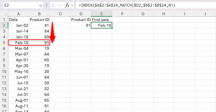
=INDEX($A$2:$A$24,MATCH($D2,$B$2:$B$24,0))

into cell E2 returns a date from cells A2 to A24 (INDEX), where the row number is determined by the first exact match (as indicated by “0” in argument c) between the value in cell D2 and the product IDs in cells B2 to B24 (MATCH).

The XMATCH Function in Excel

Microsoft Excel’s XMATCH function also tells you the position of an item in a range, but the defaults for omitted arguments differ, you can search from the bottom upwards, and you can include wildcard characters. The syntax is:

=XMATCH(a,b,c,d)

where

• a (required) is the value to look up,
• b (required) is the range of cells containing the search array, and
• c (optional) is the match mode (0 or omitted = an exact match; -1 = an exact match or the next smallest item; 1 = an exact match or the next largest item; 2 = a wildcard match), and
• d (optional) is the search mode (1 or omitted = from the top downwards; -1 = from the bottom upwards; 2 = a binary search where the array is in ascending order; -2 = a binary search where the array is in descending order).

In this example, typing:

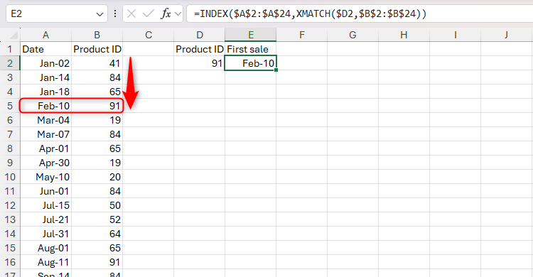
=INDEX($A$2:$A$24,XMATCH($D2,$B$2:$B$24))

into cell E2 returns the same result as the example above, where I used INDEX and MATCH, though I didn’t need to specify the match mode, as the default is an exact match. As a result, XMATCH requires you to input fewer arguments than MATCH in simple top-to-bottom lookup cases.

However, where XMATCH really trumps its predecessor is when you want to find the last match in an array by searching from the bottom upwards. This is why XMATCH has one more optional argument (a to d) than MATCH (a to c).

Here, typing:

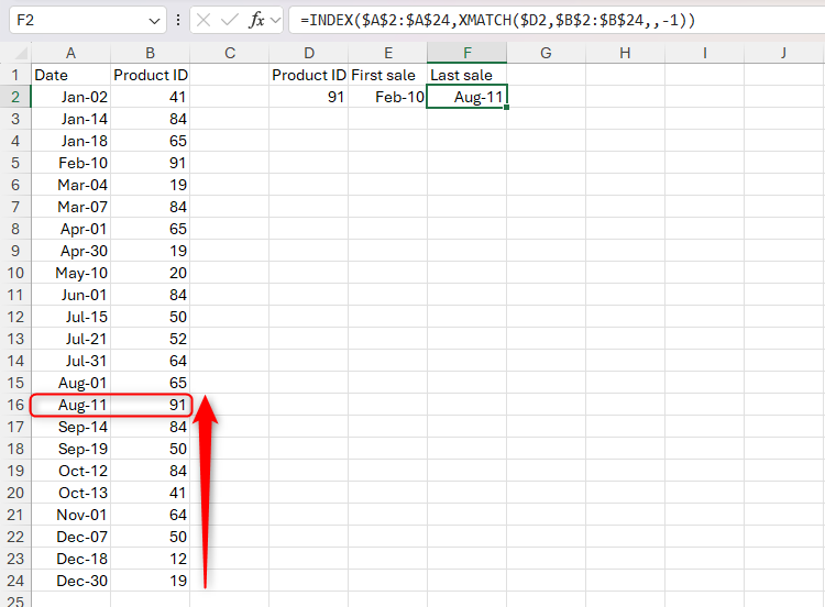
=INDEX($A$2:$A$24,XMATCH($D2,$B$2:$B$24,,-1))

into cell F2 returns the latest date from cells A2 to A24, because argument d contains “-1,” meaning the row number is determined by the last exact match between the value in cell D2 and the product IDs in cells B2 to B24. The match mode argument (c) is omitted, since the default is an exact match, and that’s what we’re looking to return.

Another benefit of using XMATCH over MATCH is that the former lets you tell Excel you’re using wildcards in the search.

Related

How You Can Use Wildcards in Microsoft Excel to Refine Your Search

Find partial matches in an instant.

Here, INDEX and XMATCH are used to find the first and last dates a product from the garden department was sold.

Notice how, in cell D2, the asterisk (*) wildcard character is used to search for a product code that starts with the letters “GD” and contains any number of characters thereafter.

Then, in cell E2, I typed:

=INDEX($A$2:$A$24,XMATCH($D2,$B$2:$B$24,2))

where “2” in the match mode argument (c) tells Excel that I’ve used a wildcard in the lookup value (a), and the search mode argument (d) has been omitted, as I wanted to search from the top downwards to find the first match.

In cell F2, I typed:

=INDEX($A$2:$A$24,XMATCH($D2,$B$2:$B$24,2,-1))

where, as well as adding the wildcard indicator for the match mode argument (c), I also typed “-1” for the search mode (d) to tell Excel to search from the bottom upwards.

To achieve the same outcome using the MATCH function, the match type must be specified as an exact match (“0”). However, since this is the default match mode for the XMATCH function, and because there’s a dedicated search mode for wildcard lookups, it’s a much more intuitive and cleaner process.

Another way to look up values in a table is by using the XLOOKUP function, an upgrade from the VLOOKUP and HLOOKUP functions. Like with XMATCH, XLOOKUP defaults to an exact match, and it lets you search from the top downwards and the bottom upwards. What’s more, XLOOKUP also lets you include an “if not found” argument, which saves the result from displaying “N/A” if the lookup value cannot be found in the array.