Key Takeaways
- Importing tables from the internet to Excel 365 is straightforward and saves time. Simply copy the web page’s URL and use the “From Web” function in the “Data” tab.
- Use the Power Query Editor to manage and transform imported data, such as removing duplicate headers or combining data from other sources.
- Customize the imported table in the Excel worksheet, adjusting formatting, column widths, and row heights. Set up automatic data refresh options if needed.
Have you found a table on the internet that you want to use in your Excel 365 spreadsheet? Manually copying the data can be time-consuming and is prone to mistakes, and if you copy and paste straight from the website, you’ll spend too much time adjusting the formatting. Instead, Excel has an in-built way to easily import the table to your spreadsheet.
Importing the Table
In your web browser, go to the web page where the data you want to import is located, and copy (using the keyboard shortcut Ctrl+C) the URL. We will use the Wikipedia page on world population as our example.
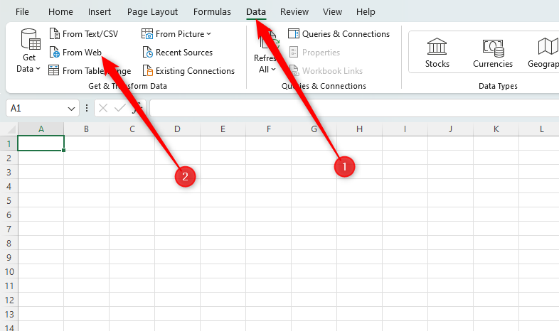
Head to the Excel workbook where you want to import the table. Open the “Data” tab on the ribbon, and in the Get And Transform Data group, click “From Web.”
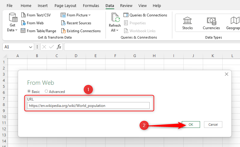
Paste (using the shortcut Ctrl+V) the URL into the dialog box that opens, and click “OK.”
Depending on the size of the web page you’re exporting from, this might take a while. Be patient!
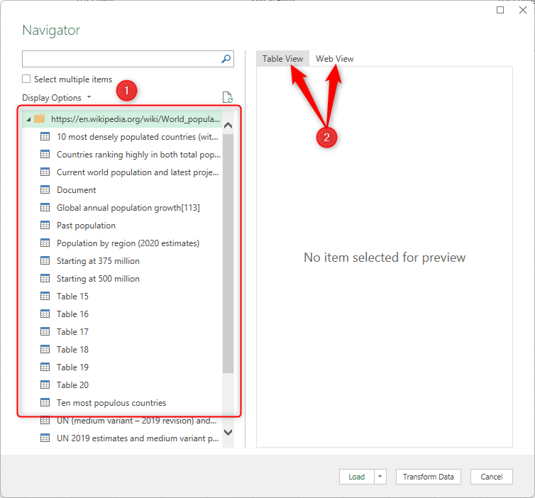
In the Navigator that opens, you can see (1) the list of tables identified on the web page, and (2) the option to view the data in Table View or Web View.
I prefer to use the Table View, as this shows roughly how the table will look when imported to Excel.
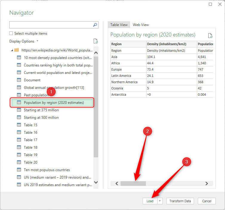
In my case, I want to import the table called “Population by region (2020 estimates),” so I will locate this in the Navigator and see how it looks in the preview. You can use the scroll bar to review the full width of the table, or simply drag the window from the edge to widen it. If you’re happy that Excel is importing the correct data, click “Load.”
If you want to choose a different place to import your data, click the drop-down arrow next to “Load”, and choose a different location. Clicking “Transform Data” will open the Power Query Editor, but we’ll get to that stage later.
Your imported table will then show in the Excel workbook you have open (in a new tab). You can split the screen to compare the original web page table and the imported table to make sure everything’s copied over correctly.
In my example, Excel has automatically formatted the data into a table and removed the national flags and all the links to other web pages, which is great—however, we can see that the header row has been duplicated, and there are some issues with spacing in the final column. Let’s look at how best to manage the imported data.
Managing the Imported Data
After you have imported the data, use the Power Query Editor to transform your data (such as removing columns), or combine your data (such as integrating info from other sources), before then loading it back onto your Excel worksheet.
The Power Query Editor also establishes and stores the connection between your Excel worksheet and the data source. Access the Power Query Editor by clicking anywhere on the imported table, opening the “Query” tab on the ribbon, and clicking “Edit.”
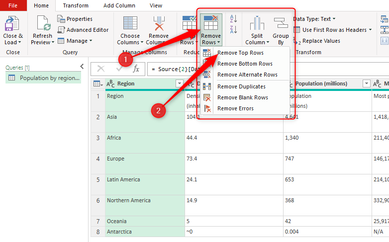
I want to remove the duplicate header row. To do this, in the Power Query Editor, I click “Remove Rows” and then “Remove Top Rows.” In the dialog box that appears, I tell Excel to remove one row.
Take some time to browse the other options in the four tabs on the ribbon. You can also see the Query Settings on the right-hand side of your window, which tracks the steps that your imported data have undergone.
Once you are happy with the shape of your data, click “Close And Load” (top-left corner), and this will take you back to your Excel worksheet with the changes updated. Again, depending on the size of the data, this may take a while to complete.
In the Excel workbook itself, you can make more specific changes to your table, such as changing the table design, shrinking the data to fit into its cell, or resizing the columns or rows.
In my case, I want to add a line break between the most populous cities and their metropolitan areas in the final column. I also want to wrap the text in each cell, increase the table’s row heights and adjust the column widths, increase the font size, and change the table design to blue. All of this can be done within the Excel workbook, as opposed to the Power Query Editor.
If you change the column width or row height, if the table updates (see below), they will revert to their imported size. To avoid this, right-click the table in your Excel workbook, hover over “Table”, and click “External Data Properties.” Uncheck the “Adjust Column Width” option.
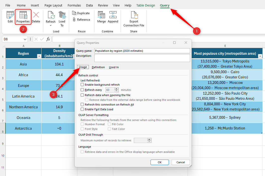
Finally, if you want to make sure your table contains the latest data, you can force Excel to refresh the imported info. Click anywhere on the table in your Excel worksheet, go to the “Query” tab on the ribbon, and click “Properties.” Then, in the Query Properties window, head to the “Usage” tab.
Here, you can choose your refreshing options:
- Enable Background Refresh: When you refresh, you can carry on with other tasks. Unchecking this option means you’ll have to wait while the refresh takes place.
- Refresh Every x Minutes: Automatically updates the data at regular intervals.
- Refresh Data When Opening The File: Forces Excel to update your table whenever you open the workbook.
- Refresh This Connection On Refresh All: Tells the Power Query Editor to make sure the link between your imported data and its source is updated.
- Enable Fast Data Load: According to Microsoft, “your query will take less time to load—however, Excel may be unresponsive for long periods of time during the upload.”
For a simple table data import, check “Enable Background Refresh” and “Refresh Data When Opening The File” (if the data won’t change very often). Choosing only these two options means that Excel will run more smoothly without constant interruptions through automatic refreshes. If you know your data is not going to change at all—for example, if you’re importing an historic sports league table—uncheck all refresh options.
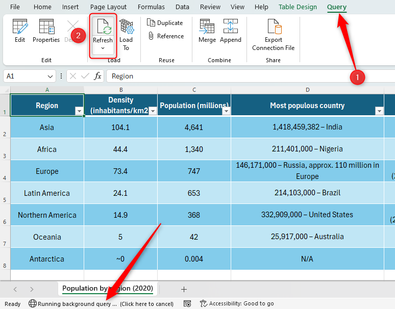
To force a manual refresh at any time, click anywhere on your table, open the “Query” tab on the ribbon, and click “Refresh”. You’ll see the status of the refresh at the bottom of your Excel window.
Now that you have successfully imported your table, you can use the data to create charts or graphs, or analyze the data using Excel’s formulas.


