Quick Links
In 2010, Microsoft added yet another technical term—Power Query—to Excel’s long list of jargon, but it’s not as complex as it sounds. In fact, once you get started, it’s not too steep a learning curve, providing you have at least a beginner’s-level understanding of Microsoft Excel.
What Is Power Query?
When first introduced to Excel, Power Query was an add-in, but given its usefulness, it has been a native tool since 2016.
In short, Power Query has one primary purpose: to save you time when handling data. More specifically, it can be used to clean up data already in Excel, import and organize data from lots of different places, or consolidate various files before loading the data to a specific location of your choice. You can also refresh the data to make sure you have the latest version.
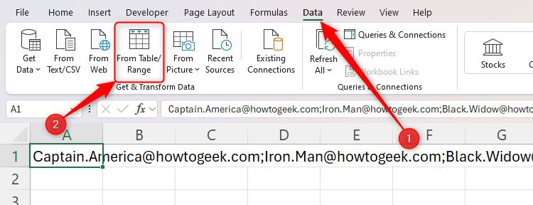
Excel’s Power Query tools can be found in the Get And Transform Data group of the Data tab.
In this article, I’ll show you how to use Power Query to clean up your data and how to import and organize data from another spreadsheet.
Using Power Query to Clean Up Excel Data
I always use Power Query to clean up data in my Excel sheets. Suppose you have copied a list of email addresses from an Outlook email’s CC field into cell A1, and you want to convert the list into a table containing first names (or titles), last names, and email addresses. While you could use Excel functions to do this, it’s much easier (and not as steep a learning curve!) in Excel’s Power Query Editor.
At this point, it’s important to note that this is just one straightforward example of how you can use Power Query to tidy up your data. If you’ve never used Power Query before, follow these steps to learn how it works in its most basic form, and then you’ll be able to experiment with other Power Query tools for tidying up more complex Excel data.
First, open the “Data” tab on the ribbon, and click “From Table/Range” in the Data group.
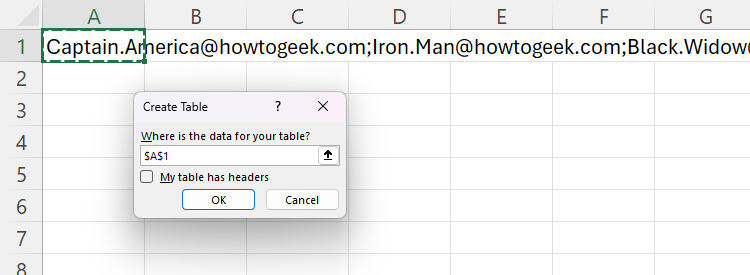
Then, in the “Create A Table” dialog box, make sure the correct cell or cells are selected, and tell Excel whether your data contains headings—in my case, it doesn’t, so I’ll leave that box unchecked—and click “OK.”
Excel will then open Power Query Editor, and this is where you can do lots of weird and wonderful things, including organizing your data.
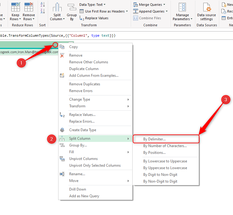
The first step is to divide each email address into its own row, so right-click the column header, hover over “Split Column,” and click “By Delimiter.” You could choose other ways to split your data, such as after a certain number of characters or between upper-case letters. In my case, however, the email addresses are separated by semicolons, so the delimiter option works.
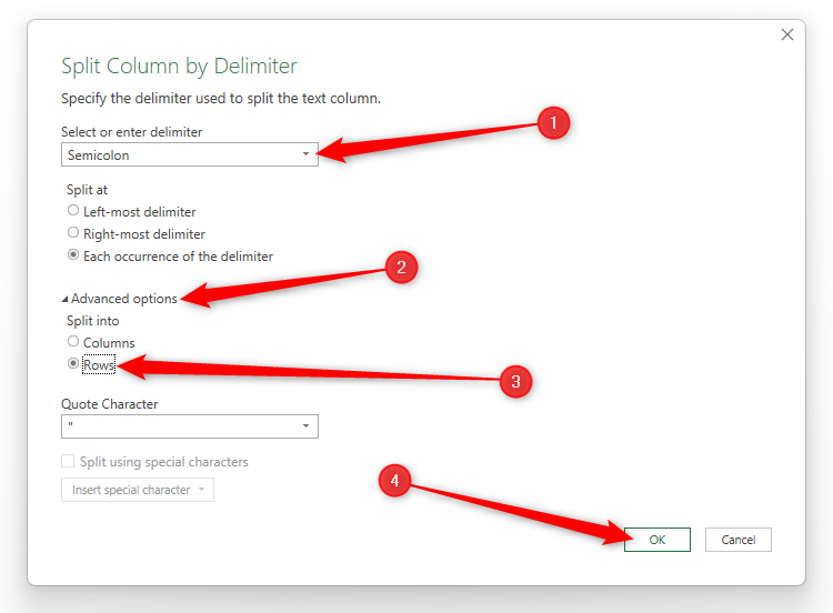
In the Split Column By Delimiter dialog box, select “Semicolon” in the drop-down list. Then, click “Advanced Options,” and check “Rows,” because you want the email addresses to be split into individual rows rather than individual columns. Now, click “OK.”
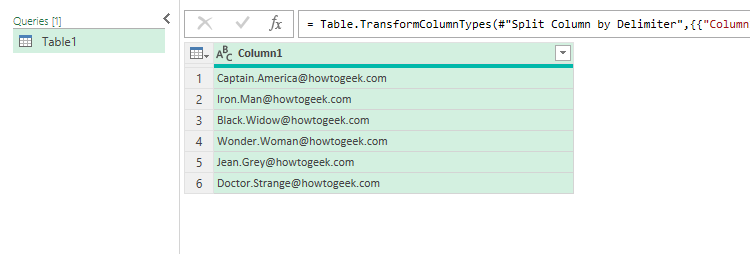
And that’s worked nicely—the email addresses have been divided into separate rows, with Power Query using the semicolon delimiter to work out when one email ended and the next began.
Notice that the Query Settings Pane on the right side of your screen records each step you take. If you mess up, just delete the relevant step to go back to where you were previously!
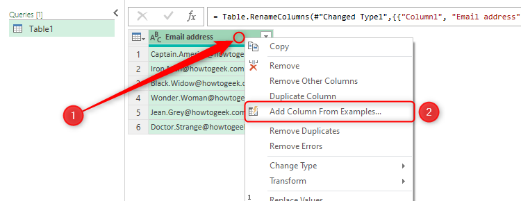
After double-clicking the column header and typing Email address, you want to extract the first name (or title) and last name into separate columns. There’s more than one way to do this, but the best method is to right-click the column header, and select “Add Column From Examples.”
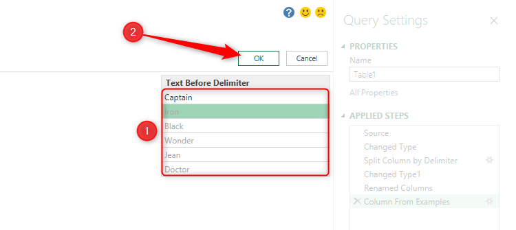
Now, since the first name in my list is Captain, I will type this into the column that has appeared on the right of my screen, and press Enter. And hey presto! Power Query Editor recognizes a pattern and suggests the remaining names to complete my column. Once you’ve checked that you’re happy with the suggestion, click “OK.”
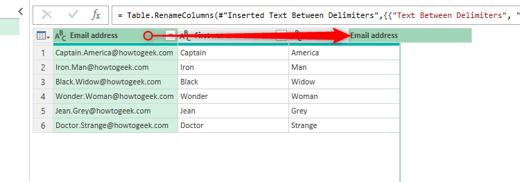
Then, follow the same process for the last name, and rename the column headers in the Power Query Editor.
You can now reorder the columns by clicking and dragging them. In my case, I want the email address column to be to the right of the names.
Before you load this new table to your spreadsheet, give it a name in the Query Settings Pane.
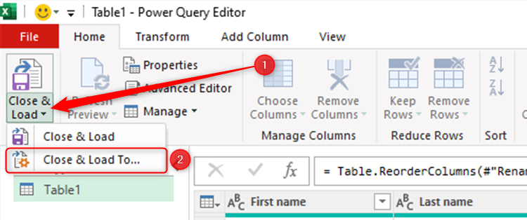
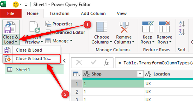
Now, click the “Close And Load” drop-down menu in the ribbon, and choose “Close And Load To.”
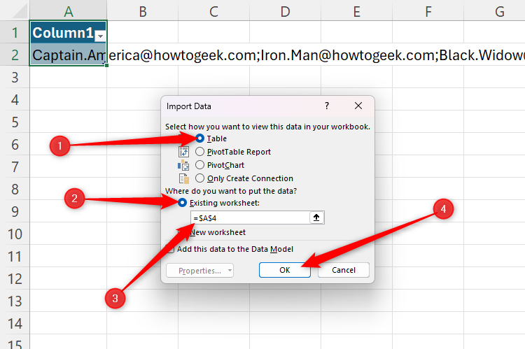
In my case, I want it to load as a table in cell A4 in the existing worksheet, so these are the options I will choose in the Import Data dialog box before clicking “OK.”
To choose a cell where the table will go, place your cursor in the field box labeled “3” in the screenshot below, and select the cell with your mouse.
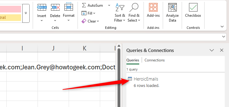
If I need to make any changes to the table, I can double-click the query in the Queries And Connections Pane.
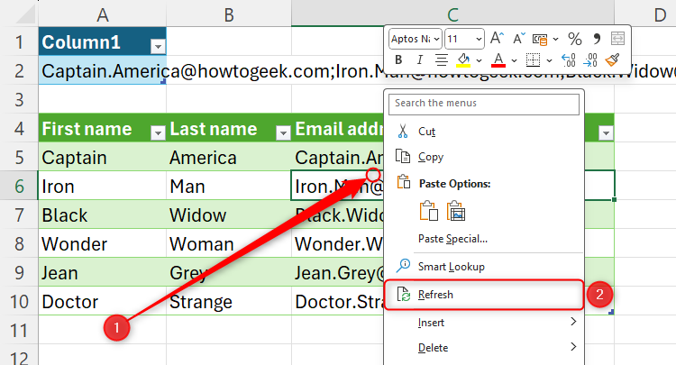
Similarly, if I amend the original list I copied from Outlook (such as adding another email address), I can update my Power Query table by right-clicking anywhere within the table and clicking “Refresh.”
Using Power Query to Import and Reorganize Data
Power Query can also be used to import data from various locations, like a PDF or a website. In this example, I’ll show you how to import and manipulate data from another spreadsheet, which is especially useful if you want to extract a very specific array of data from a large data set, or if you want to reorganize how your data is laid out.
As with the example above, I’m going to show you a very straightforward example of using Power Query for this purpose, and you can then take those skills to play around with the tool.
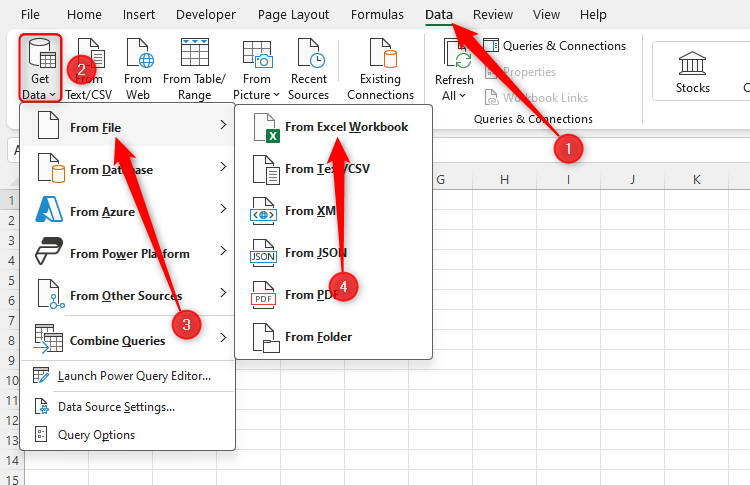
First, open the “Data” tab, and click Get Data > From File > From Excel Workbook.
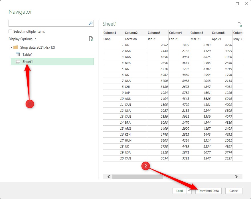
Then, use the Import Data window to locate the file from which you’re importing the data, and click “Import.” This will launch the Navigator window, which previews the data you can import from the nominated spreadsheet. In my case, I will click “Sheet 1,” which is where the data I want to import is located, and click “Transform Data.”
In the Power Query Editor that loads, I could click “Save And Load” straightaway in the top-left corner, but there are some changes to make before I do.
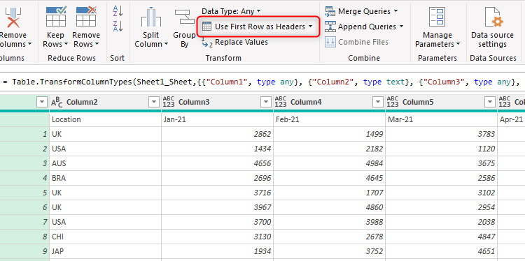
First, I need to promote my first row to the column headers, so that the first row of my spreadsheet is the first row of data. Handily, there’s a button that lets you do this in an instant: “Use First Row As Headers” in the Transform group of the Home tab.
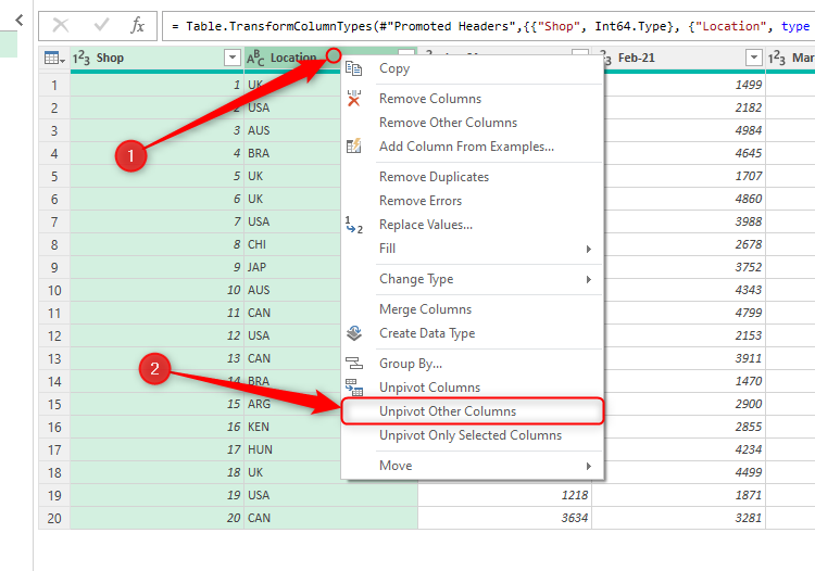
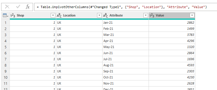
Second, I want a new row of data for each shop and each month, so that I can analyze them individually. At present, my first two columns are good as they are, so I can select them by clicking each column header while holding Ctrl. Then, I will right-click either column header, and click “Unpivot Other Columns.”
Now, each shop has its own row for each month.
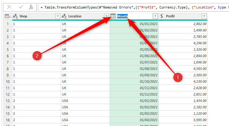
Finally, before I load this to my spreadsheet, I need to tidy up my column headings. If you want to do the same, double-click any of the headings to rename them, and click the symbol on the left of each column heading to define the data type. This will force the Power Query to flag any issues with the data, such as if one of the cells in the Month column does not contain a month.
Now, after naming your table in the Query Settings Pane on the right of the Power Query window, click Close And Load > Close And Load To, and select the location where you want the table to appear.
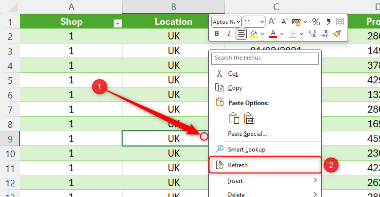
Remember, a key benefit of using Power Query over simply copying and pasting the data is that if the source data changes, you can update the rehashed data in your new spreadsheet. To make sure you’ve got the latest version of the data, simply right-click the new table, and click “Refresh.”
You can also use Power Query to import tables from the Web. For example, you might want to import a league table that is likely to change each weekend, so rather than copying and pasting the data manually and the league table quickly becoming outdated, using Power Query can help you ensure you’ve got the latest version of the data.


