Looking for a way to tidy up your spreadsheet and reduce its size without having to use dynamic range formulas like OFFSET, INDEX, or TOCOL? TRIMRANGE detects the cells your data occupies and automatically expands and contracts with it.
The Trim Ref operator is a simpler shorthand version of the TRIMRANGE function, and I’ll cover this later in the article.
The TRIMRANGE Syntax
The TRIMRANGE function has three arguments:
=TRIMRANGE(a,b,c)
where
- a (required) is the range to be trimmed,
- b (optional) determines which rows to trim (0 = no rows, 1 = leading rows, 2 = trailing rows, and 3 = both leading and trailing rows), and
- c (optional) determines which columns to trim (0 = no columns, 1 = leading columns, 2 = trailing columns, and 3 = both leading and trailing columns).
If you omit arguments b and/or c, Excel will default to trimming both the leading and trailing rows and/or columns.
Example 1: TRIMRANGE With a Sum
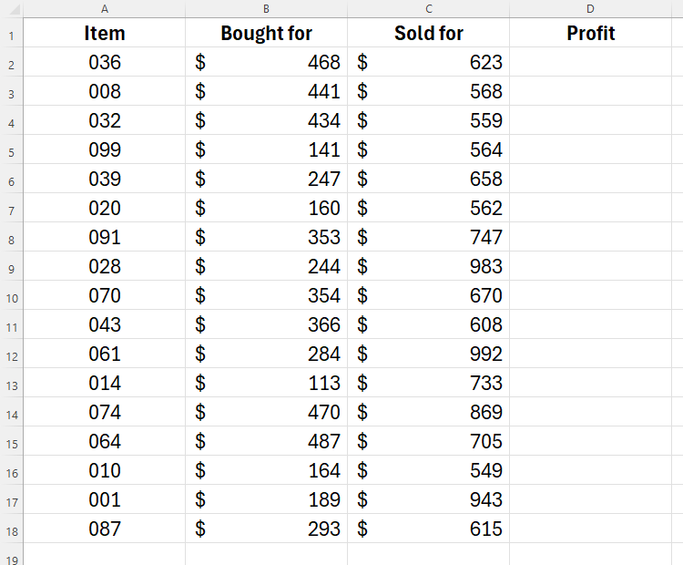
In this example, I want to subtract the values in column B from those in column C to produce a profit.
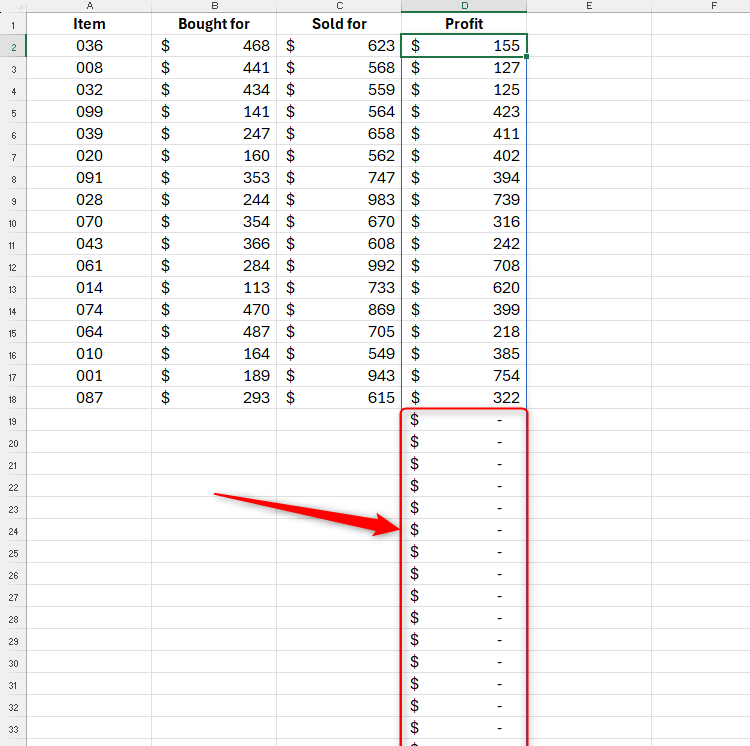
I know that I will add additional rows at the bottom at some point in the future, so I want Excel to automatically pick these up as part of the subtraction formula. To do this, I could type:
=(C2:C200)-(B2:B200)
into cell D2, as this would spill the references to the first 200 rows. However, doing this would result in an untidy spreadsheet with lots of empty calculations. What’s more, if I used whole-column references, the calculation would spill to the very bottom of the spreadsheet. This would cause there to be over a million calculations, thus significantly increasing my spreadsheet’s size and slowing it down.
Instead, I will type:
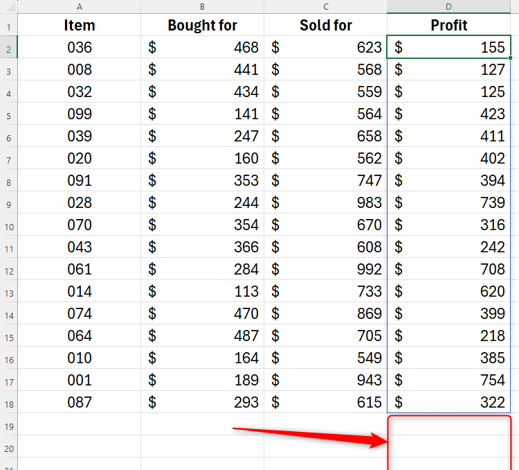
=TRIMRANGE(C2:C200)-TRIMRANGE(B2:B200)
into cell D2, which would effectively trim the redundant cells at the bottom of my data to prevent Excel from having to work too hard and keep my spreadsheet looking tidy.
I’ve omitted arguments b and c in the above TRIMRANGE references, as Excel’s default of trimming leading and trailing columns and rows works well in this example, since there are no leading blank rows or columns, and there is no data to the right of column D.
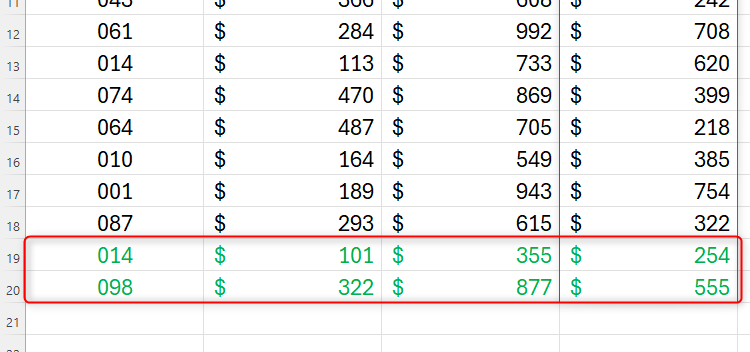
Now, when I add further rows of data at the bottom, the corresponding cells in the Profit column will calculate automatically.
Example 2: TRIMRANGE With XLOOKUP
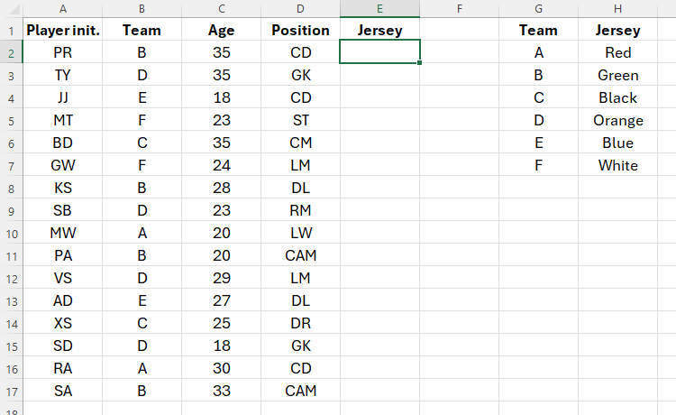
In this second example, I have a list of soccer players, and I’m going to use the XLOOKUP function to tell me which color jersey I need to provide them with, depending on the team they’re in.
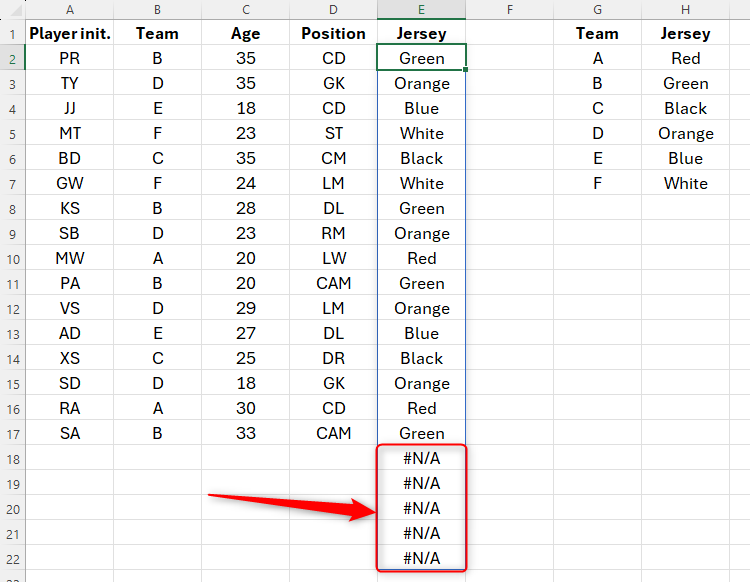
I also know that I’m going to recruit a further five players, so when I add my XLOOKUP formula, I need to extend it to row 22. So, in cell E2, I could type:
=XLOOKUP(B2:B22,$G$2:$G$7,$H$2:$H$7)
where B2:B22 is the range, $G$2:$G$7 is the lookup array, and $H$2:$H$7 is the return array. I’ve used $ symbols to tell Excel that these are absolute (fixed) cell references. However, as with the previous example, this would leave the five rows of empty data looking untidy due to the #N/A error. Also, Excel is working harder than it needs to, an issue that could affect performance if you have lots of blank rows included in your formula.
I could also use OFFSET, INDEX, or TOCOL to create dynamic range formulas, but these are much more complicated ways to achieve the same outcome as the much simpler TRIMRANGE method.
So, in cell E2, I will type:
=XLOOKUP(TRIMRANGE(B2:B22,2),$G$2:$G$7,$H$2:$H$7)
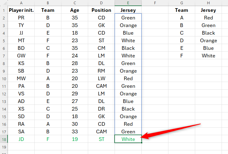
which is exactly the same formula as above, except that I’ve referenced the range (B2:B22) within the TRIMRANGE function. Notice how, this time, I’ve decided to include the second argument (“2”), which tells Excel that I want to trim trailing blank rows. However, I’ve not included a third argument, as my range only spans one column.
This time, Excel has trimmed my XLOOKUP result, and when I add more rows of data at the bottom, the cell in column E populates automatically.
Using Trim Ref Operators
Admittedly, some of the formulas I’ve used in the examples above are quite complex. This is why Microsoft has also introduced Trim Ref operators, a shorthand version of the TRIMRANGE function. In other words, the Trim Ref operators save you from having to embed TRIMRANGE within other functions. What’s more, the Trim Ref operators don’t require you to specify whether you’re trimming rows or columns, as they automatically trim both.
Using the Trim Ref operator involves adding a period (.) on either or both sides of the colon within your formula:
|
Where to Add the Period |
Which Blanks Are Trimmed |
|---|---|
|
After the colon |
Trailing blanks |
|
Before the colon |
Leading blanks |
|
Both sides of the colon |
Trailing and leading blanks |
Since the Trim Ref operators are a single “dot” in your formula, they can be difficult to spot when you’re reviewing your work or someone else’s spreadsheet. It’s something to look out for if things aren’t working as you might expect!
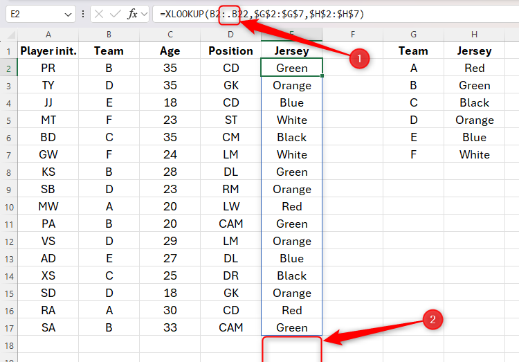
Using the same soccer player data as in Example 2, in cell E2, I will type:
=XLOOKUP(B2:.B22,$G$2:$G$7,$H$2:$H$7)
Notice how I’ve added a period after the colon in B2:.B22. This is because I want Excel to trim the trailing blanks. The screenshot below reveals the same outcome, even though I’ve used a much more straightforward formula without nesting the TRIMRANGE function within my formula.
Like when I use the TRIMRANGE function, I know I can add more rows of data at the bottom, and the XLOOKUP function will apply to that data.
Why Use TRIMRANGE and Trim Refs Rather Than Structured Tables?
You may justifiably argue that you should instead present your data in formatted Excel tables and use structured references, which automatically expand to include new data and any relevant calculations you create. In most situations, I would agree.
However, spill arrays (and some LAMBDAS) can’t go in structured tables, so in these situations, using TRIMRANGE is a handy alternative to have up your sleeve. Also, in some scenarios, you might prefer to place a range outside a structured table (for example, if you want to format your data uniquely), and the TRIMRANGE function helps you keep unstructured data tidy.
Alongside Excel’s TRIMRANGE function and Trim Refs operators, there are other ways to clean up your data in Excel, such as using Power Query or making the most of AI through Copilot.


