

Excel’s PERCENTOF function returns the percentage that a subset of data contributes to a whole dataset, saving you from having to create additional or complex formulas to generate the same outcome.
The PERCENTOF Syntax
The PERCENTOF function has two arguments:
=PERCENTOF(a,b)
where
- a (required) is the data subset that makes up part of the whole dataset, and
- b (also required) is the whole dataset.
In other words, the PERCENTOF function tells you the value of subset a as a percentage of the total dataset b.
Using PERCENTOF With a Single Value
The most straightforward use of the PERCENTOF function is to calculate the percentage of a single value against an overall total.
In this example, let’s say you’ve been asked to analyze the June performance of 14 shops in England. Specifically, your task is to work out each shop’s contribution to the overall sales total for that month.

In my example, I’ve used a formatted Excel table and structured references. As a result, my formulas are easier to parse, and if I add more data to row 16 and below, the new values will automatically be included in the calculations. If you don’t use tables and structured references, you may need to adjust your formulas so that they contain absolute references, and you’ll have to update your formulas if you add more rows of data.
To do this, in cell E2, type:
=PERCENTOF(
Then, click cell D2, which is the data subset whose contribution to the overall total you want to calculate. If you’ve used a formatted table, this will force Excel to add the column name to your formula, and the @ symbol means that each row will be considered individually within the result. Following this, add a comma:
=PERCENTOF([@[June sales]],
Finally, select all the data in column D—including the subset you selected in the previous step but excluding the column header—to tell Excel which cells make up the whole dataset. This will appear in your formula as the column name in square parentheses. Then, close the original, rounded parentheses.
=PERCENTOF([@[June sales]],[June sales])
When you press Enter, the result will display as a series of zeros. But don’t worry—this happens because the data in the percentage column is currently represented as decimals, rather than percentages.

To change these values from decimals to percentages, select all the affected cells, and click the “%” icon in the Number group of the Home tab on the ribbon. While you’re there, click the “Increase Decimal” button to add decimal places, which will help you differentiate between similar values.

And there you have it! A formatted Excel table containing a column that shows each shop’s contribution to the overall sales figures.

Related
Excel’s 12 Number Format Options and How They Affect Your Data
Adjust your cells’ number formats to match their data type.
Using PERCENTOF With GROUPBY
While PERCENTOF can be used on its own to show individual percentage contributions, it was primarily added to Excel for use with other functions. Specifically, PERCENTOF works really well with GROUPBY to further break your data down into specified categories and return the output as percentages.
Sticking with the shop sales data in the example above, let’s say your aim is to find out which counties are attracting the greatest percentage of sales.

Because GROUPBY creates a dynamic array, the function won’t work in a formatted Excel table. This is why you need to create your data retrieval table in an area of your spreadsheet that isn’t formatted as a table.
To achieve this, in cell G2, type:
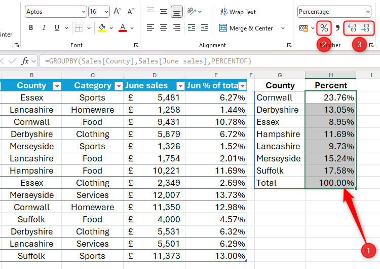
=GROUPBY(Sales[County],Sales[June sales],PERCENTOF)
where
- Sales[County] is the field in the original Sales table that will determine the grouping,
- Sales[June sales] is the field containing the values that will generate the percentages, and
- PERCENTOF is the function that will turn the raw data into comparative values.

The GROUPBY function also allows you to input another five optional fields, such as field headers, sort order, and filter array, but I’ve left these out in this example to show you how to use it with PERCENTOF in its simplest form.
When you press Enter, Excel will group the sales by county (in alphabetical order by default), presenting the data in decimalized form.

To turn these decimals into percentages, select the figures, and click the “%” icon in the Number group of the Home tab on the ribbon. You can also adjust the number of decimal places in the percentage figures by clicking the “Increase Decimal” or “Decrease Decimal” buttons in the same group of that tab.
Now, even if your data changes dramatically, the GROUPBY function will pick up these changes and adjust the categorization table accordingly.
You don’t have to stop there with your PERCENTOF fun! For example, you can embed this function within PIVOTBY to break your data down further using more than one variable, before showing the output as percentages.

")
