Summary
- Applying direct formatting to spilled arrays in Excel could cause issues if the data changes shape or size.
- Formula-based conditional formatting rules allow for automatic formatting adjustments when the data parameters change.
- Placing a dollar symbol before the column reference lets you apply the rules to all the rows in the data.
In Excel, you can apply direct formatting to cells’ values or backgrounds to make the spreadsheet easier to read. However, when an Excel formula returns a set of values—known as a spilled array—applying direct formatting will cause issues if the size or shape of the data changes.
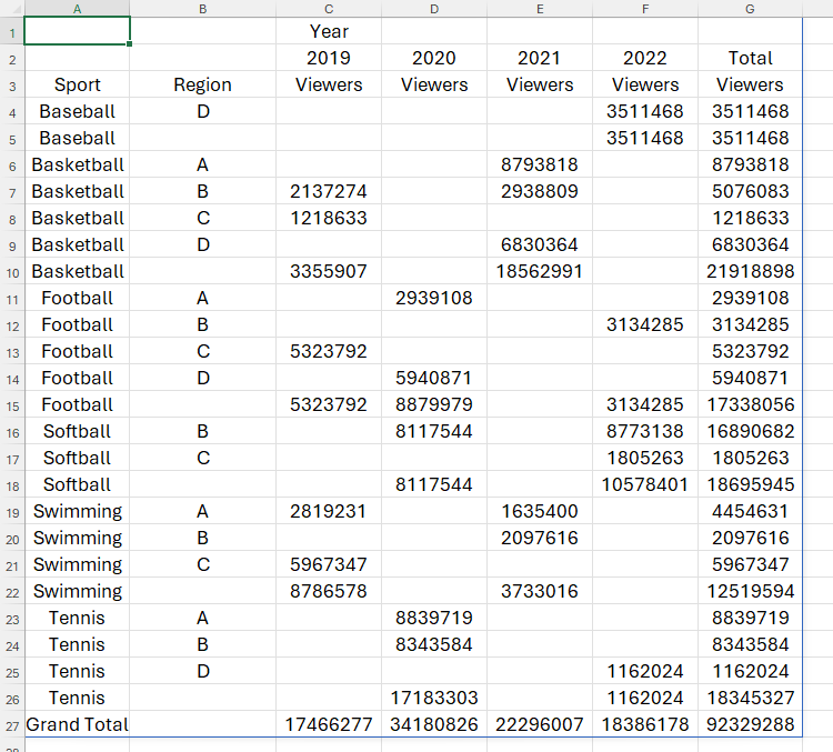
Let’s say you have this spreadsheet containing the spilled result of a PIVOTBY formula, which shows the number of viewers per sport across various regions over four years.
To follow along as you read, download a copy of this Excel workbook. After you click the link, you’ll find the download button in the top-right corner of your screen.

Related
Because the PIVOTBY function doesn’t include an argument that lets you format the result, distinguishing between the header rows, data rows, subtotal rows, and grand total row is difficult.
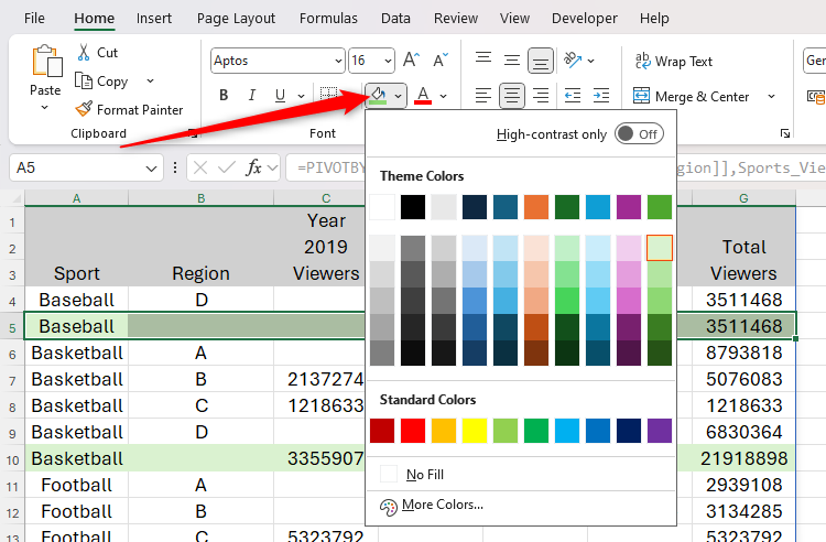
At this stage, you might be tempted to apply direct formatting—via the Font group of the Home tab on the ribbon—to visually separate the different types of rows in the data.
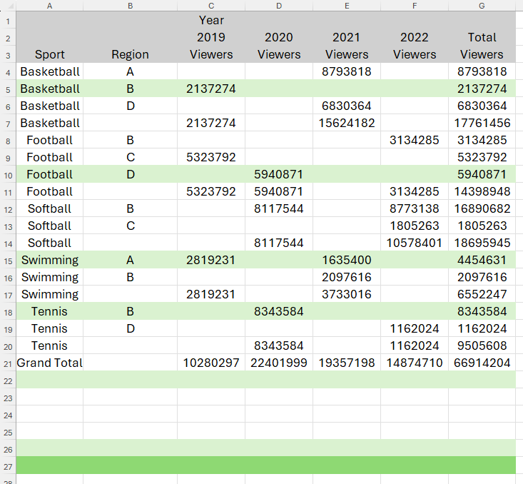
However, if you later modify the parameters in the PIVOTBY formula, or if the result grows or shrinks due to changes in the original data, the direct formatting you applied won’t adjust accordingly. This is because direct formatting in Excel is linked to the cells, rather than the data they contain. See the confusion this could cause in the screenshot below, where the data has shrunk, but the direct formatting is still applied to the same rows.
Instead, you should use conditional formatting, which allows you to format the cells and rows according to their values.

Related
I Use Conditional Formatting in Most Spreadsheets: Here’s Why
Conditional formatting is a non-negotiable.
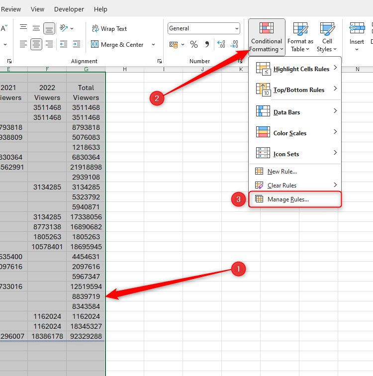
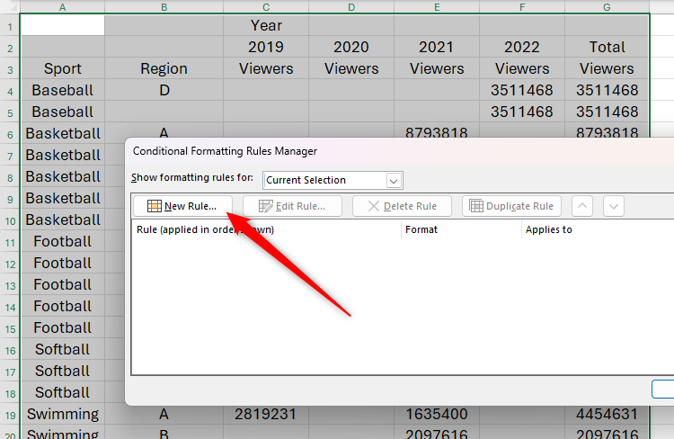
Select all the data—plus some extra rows at the bottom to allow for vertical growth—and in the Home tab on the ribbon, click Conditional Formatting > Manage Rules.
Next, in the Conditional Formatting Rules Manager dialog box, click “New Rule.”
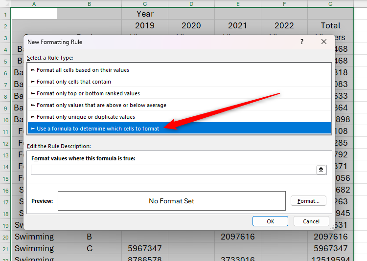
For each of the rules you’re going to create to format your spilled array, you’ll need to use a formula. So, in the Select A Rule Type area of the New Formatting Rule dialog box, select the final option, “Use A Formula To Determine Which Cells To Format.”
The first rule you want to create relates to the header rows. Specifically, you want those cells to adopt a gray background.
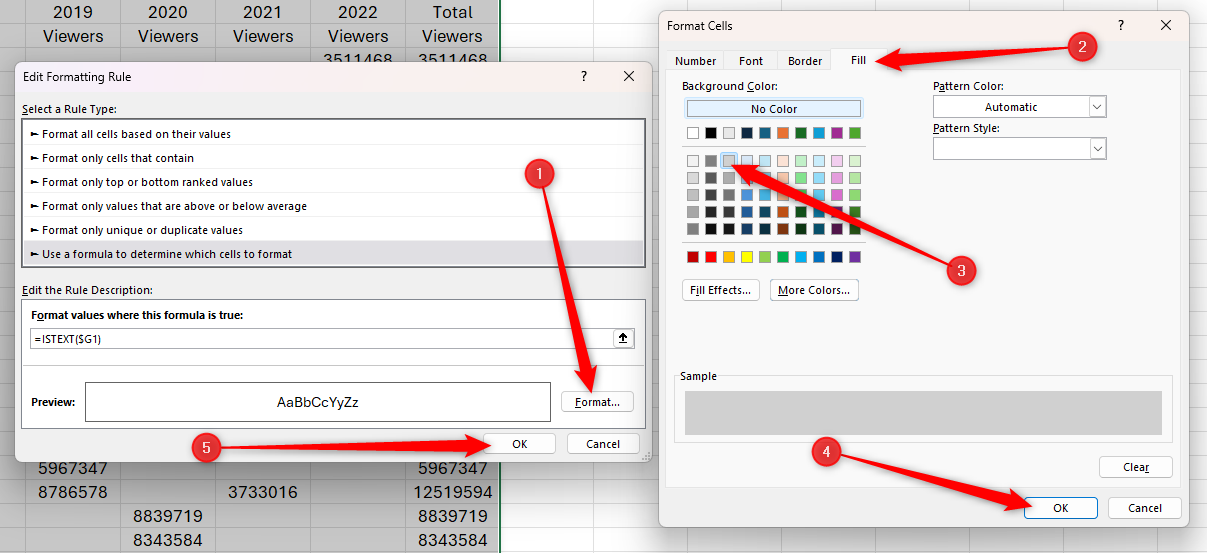
To achieve this, take a moment to identify what makes the header rows unique from the other rows in your table. In this case, the header rows are the only rows that don’t contain numbers in column G. So, in the formula field, type:
=ISTEXT($G1)
Since the ISTEXT function treats blank cells and cells containing text as a text value, the conditional formatting rule will consider cells G1 to G3 as containing text, with the remaining cells in column G containing number values.
Importantly, adding a dollar ($) sign before the column reference—also known as a mixed reference—fixes the conditional formatting to this column, while allowing Excel to apply the rule to the remaining rows.
After typing a cell reference, rather than typing the dollar sign manually, press F4 to toggle between absolute references (for example, $G$1), mixed references (for example, $G1 or G$1), and relative references (for example, G1).

Related
How to Use Relative, Absolute, and Mixed References in Excel
Save time and reference the correct cells when creating formulas in Excel.
Finally, because you initially selected data in columns A to G, the conditional formatting will apply to the whole row where the condition is met.
Now, click “Format” to select the formatting for the header rows. In this case, you want them to be colored gray. Then, click “OK” in the Format Cells and Edit Formatting Rule dialog boxes.
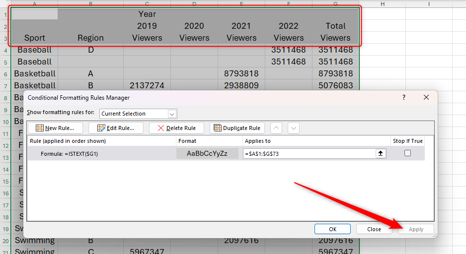
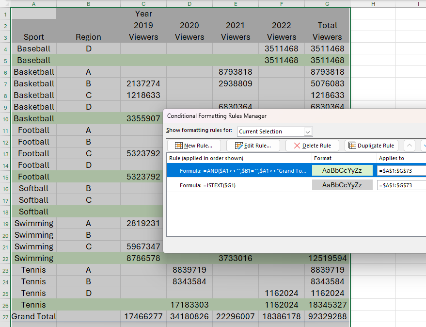
When you click “Apply” in the Conditional Formatting Rules Manager dialog box, you’ll see that only the rows in which column G contains blank cells or text—in other words, the header rows—are filled in gray.
Next, you want to format the subtotal rows so that they adopt a light green fill.
Again, carefully review the data to see what conditions you can use to apply the formatting to these rows only. In this case, the subtotal rows contain text in column A but nothing in column B. Also, since the grand total row also meets these criteria, you need to exclude any cells in column A containing the words “Grand Total.”
With the Conditional Formatting Rules Manager dialog box still open, click “New Rule,” and select the option that lets you use a formula to format the cells. This time, in the formula field, type:
=AND($A1"",$B1="",$A1"Grand Total")
where
- The AND function lets you specify more than one condition within the parentheses,
- $A1>”” tells Excel to look for cells in column A that do not contain () blank cells (“”),
- $B1=”” tells Excel to look for cells in column B that do contain (=) blank cells (“”), and
- $A1>”Grand Total” tells Excel to exclude () any cells in column A that contain the text “Grand Total.”
As with the previous rule, remember to insert the $ sign before the column references to allow Excel to apply the same rule down all the selected rows.
Now, click “Format” to choose the light green fill color, and after closing the Format Cells and Edit Formatting Rule dialog boxes, click “Apply” to see the subtotal rows filled in light green.
Finally, you want the cells in the grand total row to be filled with a bolder green.
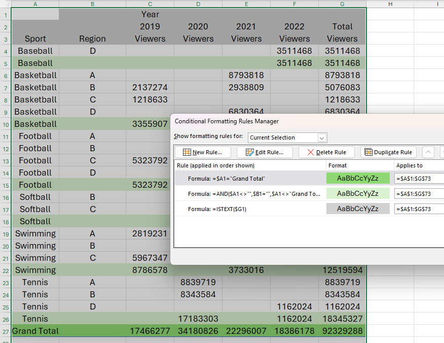
Since the grand total row is the only row that contains the words “Grand Total” in column A, this is the criterion you can use for the conditional formatting. In the Conditional Formatting Rules Manager dialog box, click “New Rule,” and select the final option in the Select A Rule Type list. Now, in the formula field, type:
=$A1="Grand Total"
Next, click “Format,” and select a bold green fill color to apply to the cells that match this criterion. Now, when you close the Format Cells and Edit Formatting Rule dialog boxes, and click “Apply” in the Conditional Formatting Rules Manager dialog box, you’ll see that your grand total row has adopted this formatting.
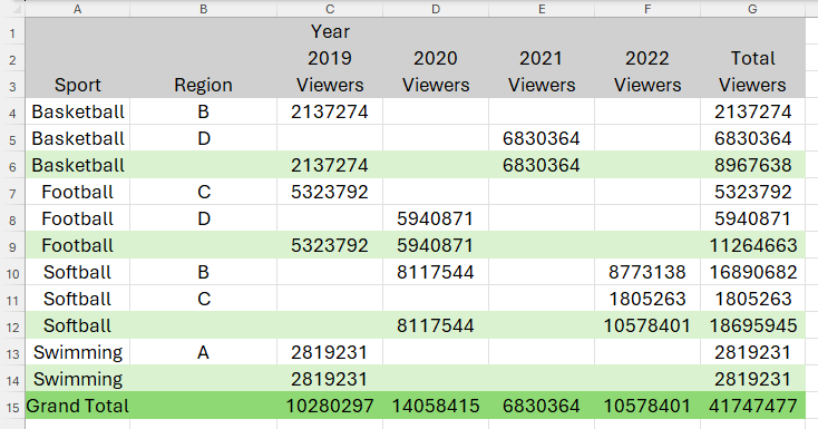
Now that you’ve applied all your rules, click “Close” in the Conditional Formatting Rules Manager dialog box. Then, adjust some of your data in the original table, and see the spilled result and its formatting update accordingly.
In this example, even though I removed 12 rows from the original data table, the spilled PIVOTBY result is still correctly formatted, with the header rows colored gray, the subtotal rows colored light green, and the grand total row colored bold green.
If you need to make any changes to the rules you have created and applied, simply select any cell in the data, and click Conditional Formatting > Manage Rules to relaunch the Conditional Formatting Rules manager. Then, double-click a rule to change its conditions.


