Does your large spreadsheet contain lots of blank rows that serve no purpose? Don’t waste time removing these empty rows manually! Instead, use this tip to ensure you don’t miss any rows or accidentally delete the incorrect rows.
The Method to Avoid: Ctrl+G
Many quick tip videos and tutorials suggest you should delete blank rows in your spreadsheet by pressing Ctrl+G (to launch the Go To dialog box), clicking “Special,” checking “Blank,” and then clicking Delete > Delete rows.
However, this method deletes all rows containing any blanks, whereas our aim is to delete the rows containing all blanks. In other words, if you use this method, there’s a good chance you’ll lose some of your data. Don’t be fooled by its apparent simplicity!
Use Excel’s COUNTBLANK Formula
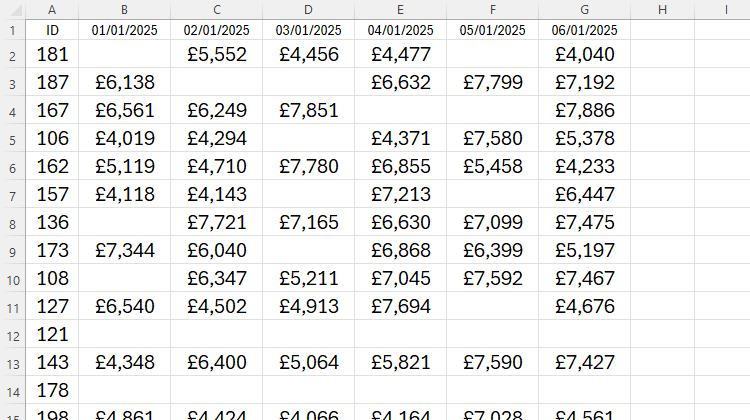
This spreadsheet contains hundreds of rows of data. Some rows contain blank cells but data in other cells, while some rows contain no data altogether. Your aim is to remove the rows containing no data at all, but keep the rows containing any data.
Step 1: Add a Filter Row
The first step is to add a filter row at the top of your data.
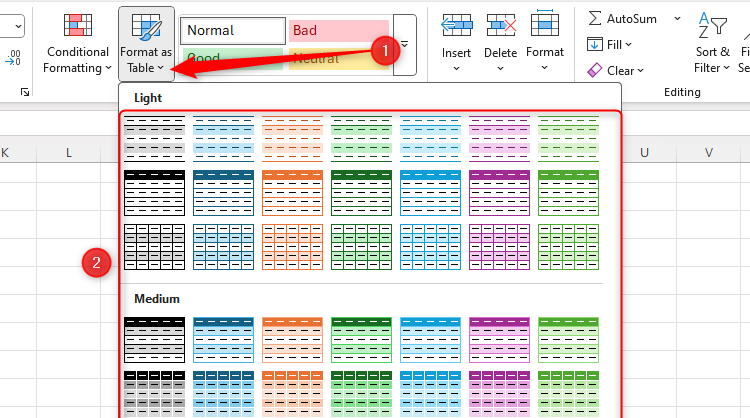
There are two ways to achieve this. First, select any cell in your data, click “Format As Table” in the Home tab on the ribbon, and choose a table design.
When you click “OK” in the Create Table dialog box, a filter row will be added automatically at the top of your data.
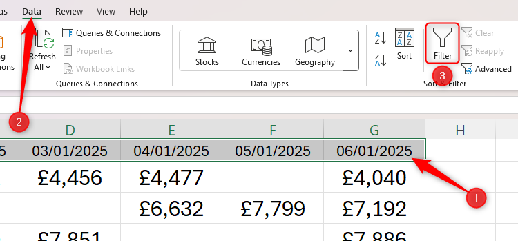
While the method above is the best approach, if you don’t want to reformat your data into a table, select the cells in your top row that contain information, and click “Filter” in the Data tab on the ribbon.
Step 2: Add a Blanks Column
In row 1 of the column to the right of your table, type the column header Blanks.
If you formatted your table, Excel will automatically extend the formatting and the filter to the new column you just created. If you didn’t format your data into a table, you’ll need to remove and then re-add the filter to incorporate this additional column.
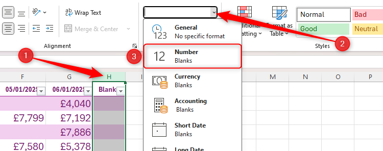
Next, select your new column by clicking the column letter above where you typed your header (in my case, I’ll click “H”). Then, in the Number group of the Home tab on the ribbon, click the Number Format drop-down menu, and click “Number.”
Step 3: Count the Blanks
Now, in the first cell under the column header, type:
=COUNTBLANK(
Next, press the Left Arrow key once, and then press Shift+Home. This will select the whole row to the left of the active cell, thus completing your formula’s parameters. Then, close the parentheses.
=COUNTBLANK(Table1[@[ID]:[06/01/2025]])
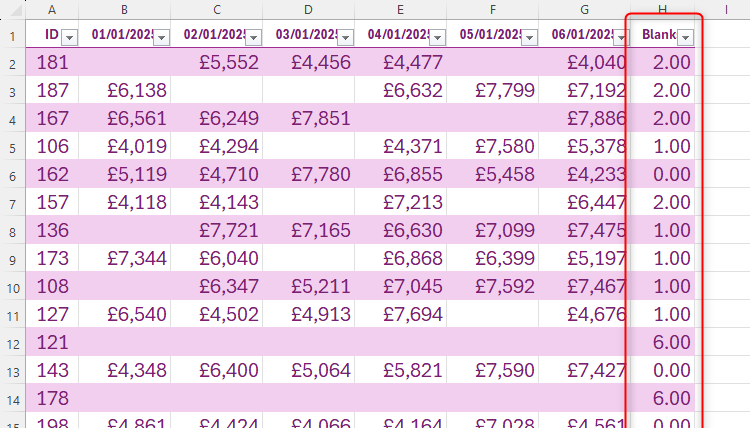
As you can see in my example above, the formula includes all columns from the ID in column A to the final date in column G. If you aren’t using a formatted table, your formula will contain direct cell references (for example, A2:G2) rather than structured table column references.
When you press Enter, you’ll see the total number of blank cells in that row. If you’re using a formatted table, this formula will be applied automatically to the remaining rows in your table.
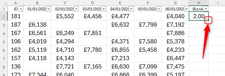
If you’re not using a formatted table, double-click the fill handle in the bottom-right corner of the cell containing the formula you just typed, and see the remainder of the column populate with the number of blanks in each row.
Step 4: Filter and Delete
Finally, you can now use the filter you added earlier.
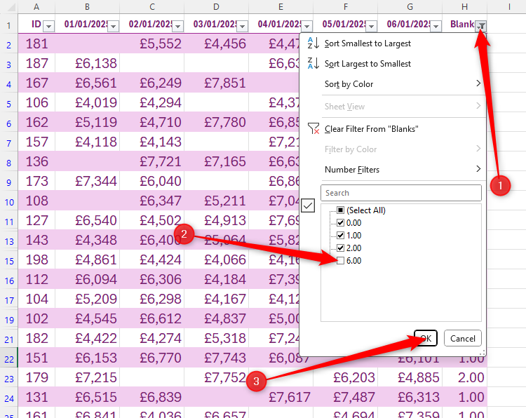
The first option is to hide the rows containing all blanks by unchecking the highest number in the filter drop-down. In my case, I want to hide the rows containing six blanks.
When I click “OK,” even though the rows are still stored within my spreadsheet, they’re hidden from view due to the filter I applied.
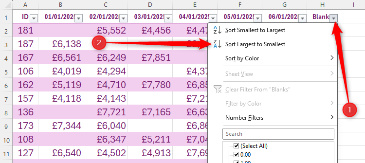
Alternatively, sort the data by the Blanks column by clicking “Sort Largest To Smallest.”
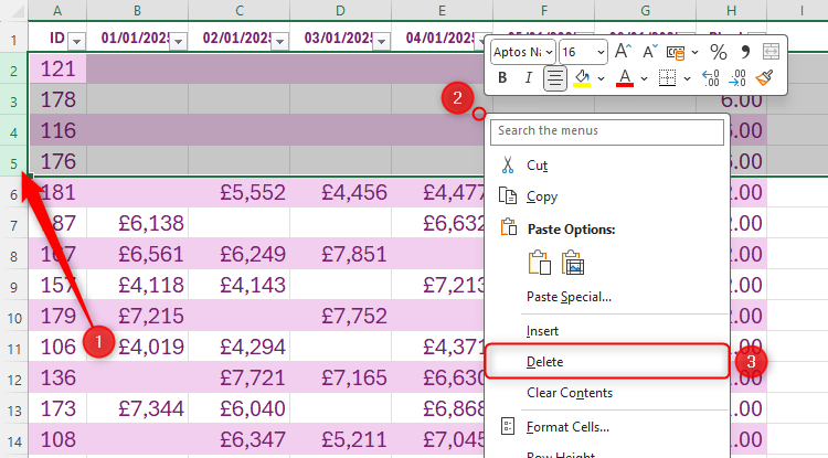
With the blank rows now at the top of your table, you can select them all, right-click the selected cells, and click “Delete.”
Deleting blank rows in Excel is just one way to clean up your spreadsheet. Indeed, there are many useful ways to rearrange your Excel data, resulting in an impressively tidy workbook.


