Most formulas in Excel return a single-cell result. However, if an Excel formula returns a set of values, the result will spill over to neighboring cells.
Spilling and dynamic array formulas are not supported in Excel 2019 or earlier.
The Definitions You Should Know First
Before I show you examples of spilling in action, here are the definitions of some related Excel terms in this guide:
- Spilling: When Excel formulas return a set of values (also known as an array).
- Array: A set of data within a range of cells. For example, if cells A1 to A20 contain data, A1:A20 is the range, and the data within that range is the array.
- Function: A pre-defined formula that performs a calculation when used in a formula.
- Formula: A combination of functions, cell references, values, operators, and names that, when used together following the equals (=) sign, returns a result
- Dynamic array formula: A formula that is capable of returning an array.
- Spilled array formula: A formula that is currently returning a spilled array.
Examples of Spilling
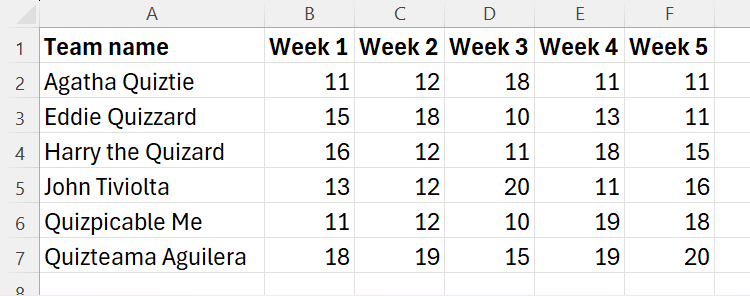
First, let’s look at a straightforward example of spilling in Excel. This Excel spreadsheet contains six quiz teams and their scores for weeks one to five.
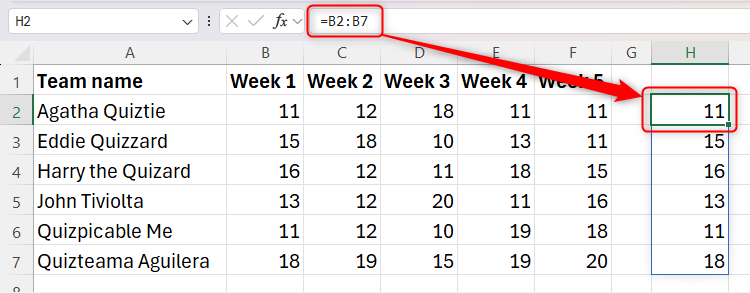
Because
=B2:B7
is a dynamic array formula, typing it into cell H2 returns a spilled array covering H2 to H7. Notice how, when I select cell H2, Excel places a temporary border around those cells to remind me that it is a spilled array.
If I were to type values into cells H3 to H7, this would interfere with and break the spilled array that Excel has just created, resulting in a #SPILL! error. I’ll talk more about #SPILL! errors shortly.
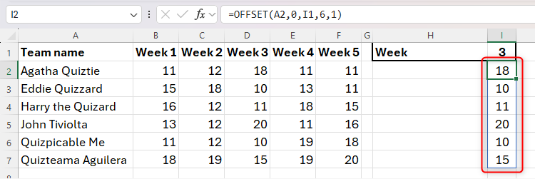
Now, however, I want to make more practical use of this type of result by using the OFFSET function. In this case, I want Excel to tell me what each team scored in a given week, depending on the number I type into cell I1.
To do this, in cell I2, I will type
=OFFSET(A2,0,I1,6,1)
because I want Excel to start at cell A2, stay on the same row, move across the number of columns I typed in cell I1, and return a result that is 6 rows down and 1 column across. Since Excel is returning an array that is 6 rows in height, even though I only typed the formula into cell I2, the result spills from cells I1 to I7.
To tidy up my data retrieval table, I also want to add the team names to column H. To do this, I will type
=A2:A7
into cell H2, which also produces a spilled array. I’ve also applied some formatting to improve the spreadsheet’s readability.
One benefit of using dynamic array formulas such as those above is that if the data were to change or be rearranged, the spilled arrays would adjust accordingly.
In a final example, I’m going to use the XLOOKUP function to produce a spilled array. My aim is to display a certain team’s set of results over the entire five-week period, with the team in question depending on the value in cell I1. First, I will type the dynamic array formula
=B1:F1
into cell H3 to produce the spilled array of week numbers in cells H3 to L3.
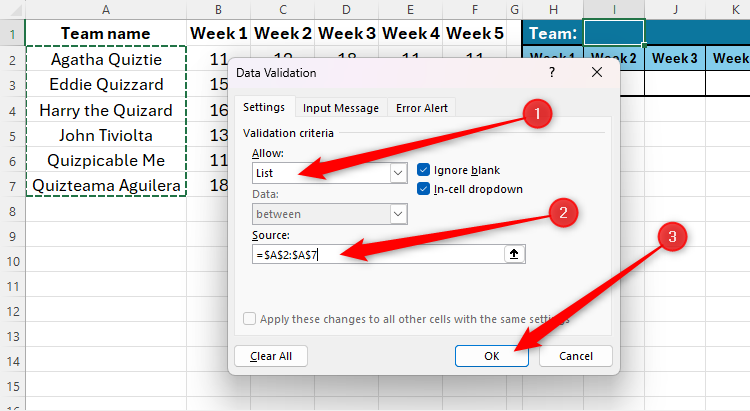
Now, I will create a drop-down list in cell I1 containing the team names listed in cells A2 to A7. To do this, I will click Data > Data Validation, choose “List” in the “Allow” field, and select cells A2 to A7 to define the source of the list, before clicking “OK.”
Finally, I can use the XLOOKUP function to return the scores for my selected team across the five weeks. In cell H3, I will type:
=XLOOKUP(I1,A2:A7,B2:F7)
because I want Excel to take the team name in cell I1, match it to a team name in the range A2 to A7, and return the corresponding array from columns B to F. Since the result is five columns wide, it is displayed as a spilled array across cells H3 to L3. In this case, I selected team Quizpicable Me from my drop-down list in cell I1.
Other functions that typically result in a spilled array include FILTER, SORT, UNIQUE, and RANDARRAY.
Referencing a Spilled Range
To reference a spilled range, use the spilled range operator (#) after the range within the dynamic array formula. Using the same example as above, I want to display a total score for a given team based on the spilled array in cells H3 to L3.
So, typing
=SUM(H3#)
into cell L4 tells Excel to sum the array in the spilled range starting at H3.
Fix Common #SPILL! Errors
Certain situations will cause Excel to return the #SPILL! error. Here’s what to look out for if this happens in your spreadsheet, and also what you can do to fix the issue:
|
Cause of the #SPILL! Error |
Ways to Fix the Error |
|---|---|
|
The spilled array crosses over a merged cell. |
Select the merged cell, and click “Merge And Center” in the Alignment group of the Home tab to unmerge the cell. |
|
Something is blocking the cells where the spilled array is trying to go. |
Delete or move the data in the cell that is blocking the spilled array. |
|
The range in the dynamic array formula extends beyond the worksheet’s edges. |
Review the dynamic array formula to ensure that the cell references are accurate. |
|
The dynamic array formula is used within a formatted Excel table. |
Move the dynamic array formula to a location outside the formatted table. Alternatively, convert your formatted Excel table to an unformatted range by selecting one of the cells within the table, and clicking “Convert To Range”) in the Tools group of the Table Design tab. |
|
The dynamic array formula has caused Excel to run out of memory. |
Reference a smaller range within your dynamic array formula. |
|
The spilled range is not known, as the dynamic array formula contains a volatile function. |
Dynamic array formulas do not work with spilled arrays of unknown lengths. Unfortunately, the only way to overcome this issue is to avoid using dynamic array formulas that create arrays of variable lengths. |
If your dynamic array formula references a whole column, you can use the TRIMRANGE function to tell Excel to discount empty rows, essentially trimming the data to include only the necessary cells.


