Excel is well known as a program that allows you to create complex tables of data. However, some people are less familiar with a special type of reference that comes with these tables: structured references.
Structured references can be used in Excel 2016 or later, including Excel 365.
What Is a Structured Reference?
Direct cell references in Excel link one cell to another using the column and row header labels. For example, cell A1 is in the first column and first row, while cell C10 is in the third column and tenth row.
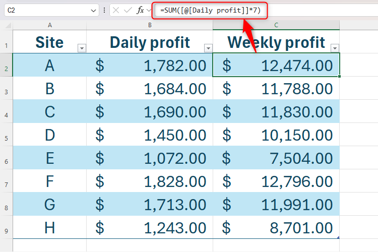
On the other hand, rather than using the column and row header labels, structured references use table and column names. In the example below,
=SUM([@[Daily profit]]*7)
takes the values in each of the cells in the column named “Daily profit” and multiplies them by seven.
Using Structured References Within a Table
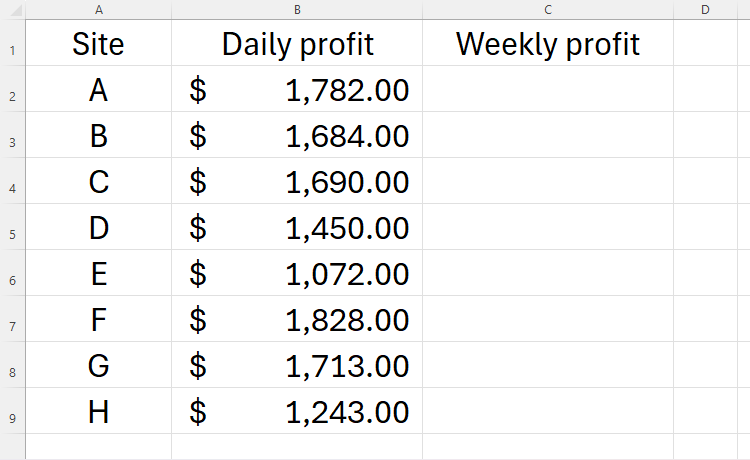
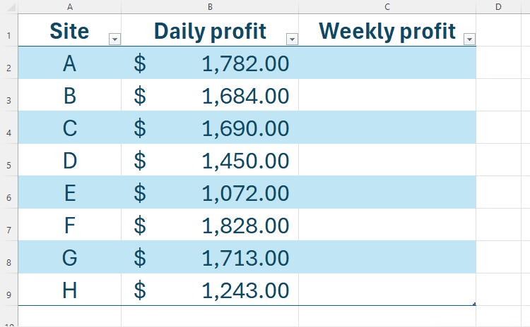
To use structured references within your table, as in the example above, you first need to add some data to your Excel worksheet, with column names included across the top of this data. If you don’t add column names, Excel will default to Column 1, Column 2, and so on, which is far less clear when you want to use the headers in formulas later on.
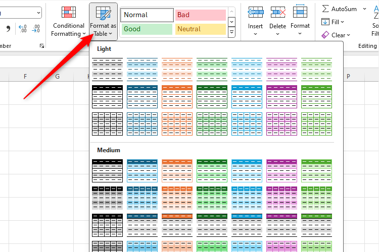
Before you use any of the data to create calculations, select a cell within your data, and click “Format As Table” in the Home tab on the ribbon. There, select the design that works best for you.
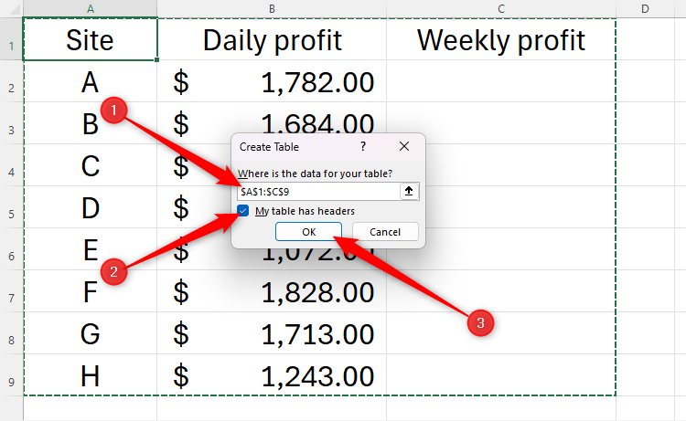
Now, use the Create Table dialog box to verify that all your data is selected, check the “My Table Has Headers” checkbox, and click “OK.”
Now that your data is in a formatted Excel table, you’re ready to use structured references.
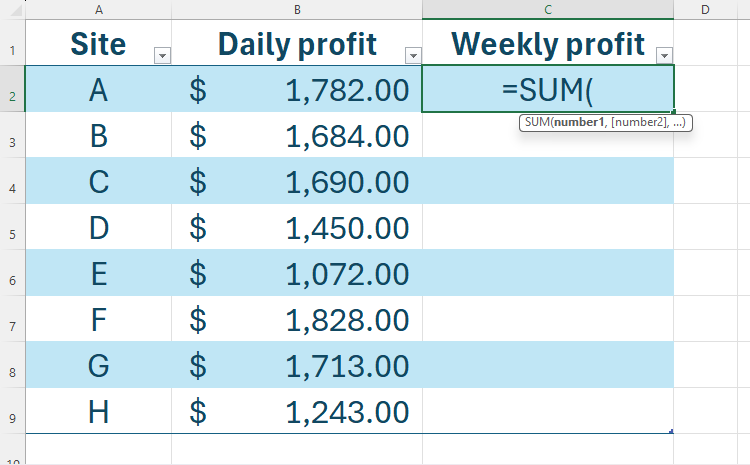
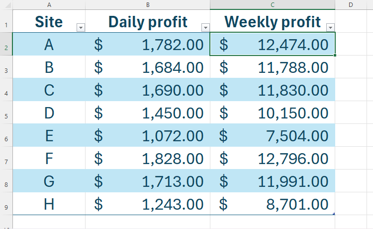
In my example, I will select cell C2 (the first cell where I want to create a calculation), and type:
=SUM(
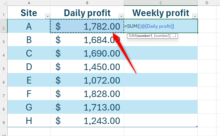
Now, I will click the first cell containing data in my “Daily profit” column, and Excel will insert a structured reference to that column.
=SUM([@[Daily profit]]
The square parentheses are Excel’s way of indicating that it’s using a structured reference, and the @ symbol (also known as the intersection operator) means that the calculation will be applied respectively to each row within the table.
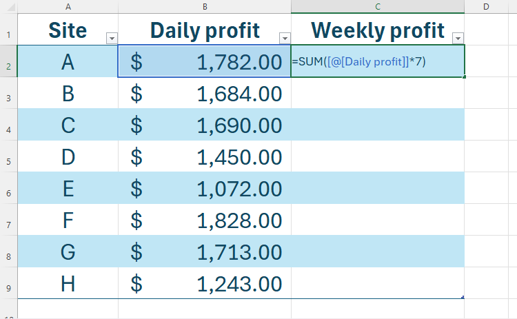
Finally, I need to multiply the values in the “Daily profit” column by seven to generate the weekly profit, and close the round parentheses.
=SUM([@[Daily profit]]*7)
When I press Enter, the formula will copy automatically to the remaining cells in the “Weekly profit” column.
If I manually removed the @ symbol, the calculation in the “Weekly profit” column would sum the whole of the “Daily profit” column, and multiply that total by seven.
Using Structured References Outside a Table
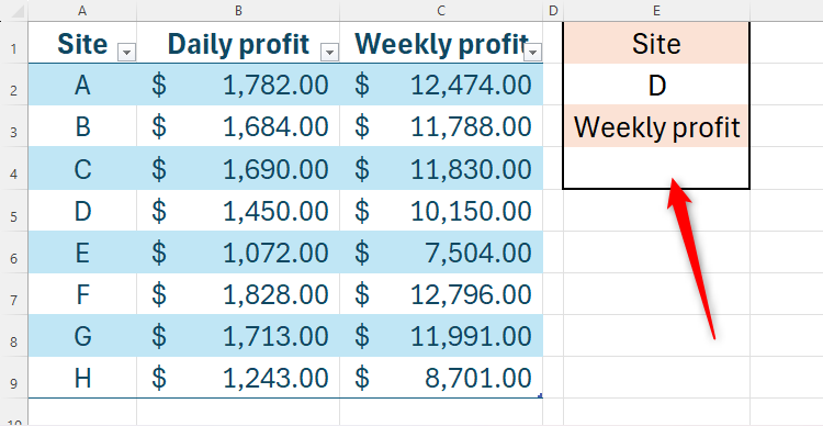
Structured references are also used within formulas outside an Excel table that reference table data. In this example, I will use the XLOOKUP formula to generate a weekly profit in cell E4 based on the site stated in cell E2.
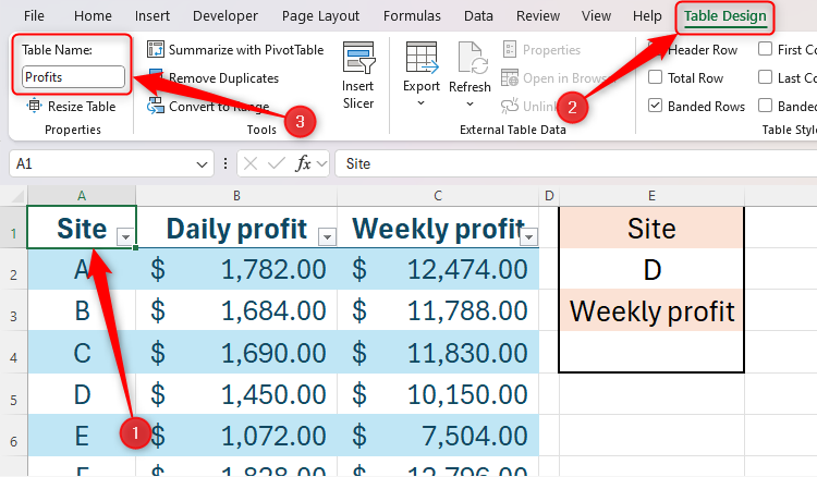
The first step is to name the table. Otherwise, Excel will name my data Table1, which could be confusing if there are several tables in my workbook. In fact, it’s good to get into the habit of naming your tables whenever you create them in Excel, even if you don’t intend to reference them anywhere else in your spreadsheet.
To do this, I will select any cell within the table, open the “Table Design” tab on the ribbon, and type an appropriate name in the Table Name field. In my case, I’ll call my table “Profits.”
There are certain rules you must follow when naming your table:
- Your table name must start with a letter, an underscore (_), or a backslash (\).
- The rest of the table name can be a combination of up to 255 letters, numbers, periods, and underscores.
- Your table can’t be called “C,” “c,” “R,” or “r,” because these are used for other purposes in Excel.
- Your table also can’t be the same as a cell reference, such as A1 or $A$1.
- Try to keep the table name to one word so that it’s easy to reference. However, if you must use more than one word, use an underscore (not a space) between each word.
- Make sure the table name has not been used elsewhere in your workbook.
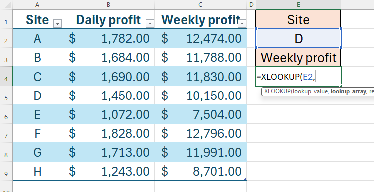
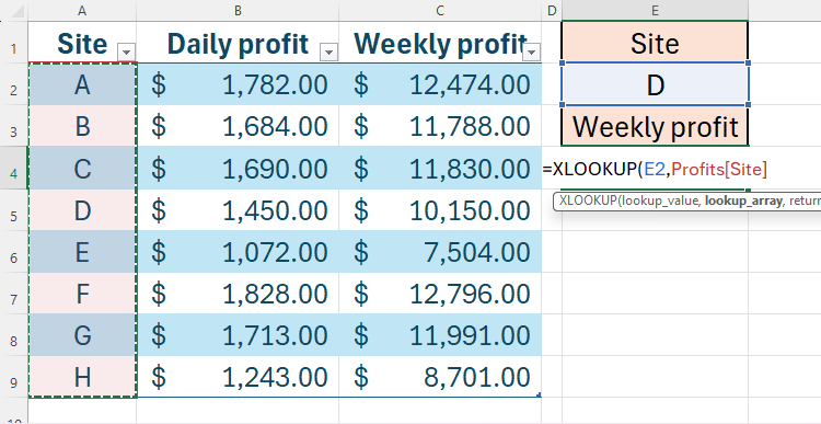
Now, in cell E4, I can start my XLOOKUP formula by typing:
=XLOOKUP(E2
Then, I need to select the lookup array, which is cells A2 to A9. Notice how my formula automatically converts this to a structured reference, with “Profits” being the table name I created earlier and “Site” being the column header.
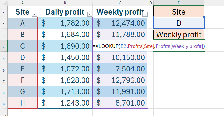
=XLOOKUP(E2,Profits[Site],
Finally, I can select the return array, which is cells C2 to C9, and close my round parentheses. Again, Excel turns this into a structured reference for me.
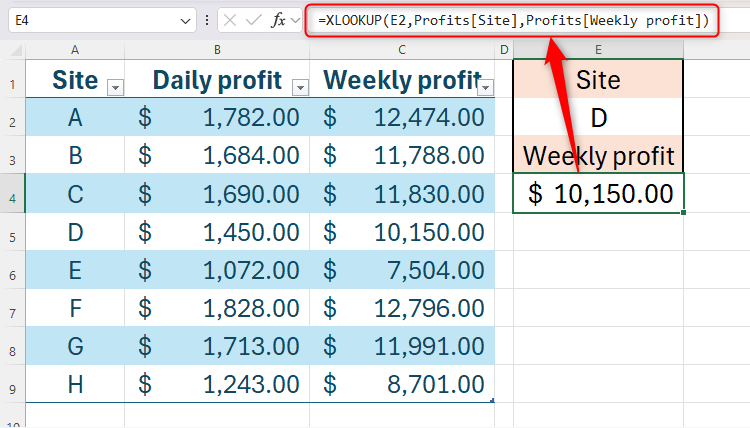
=XLOOKUP(E2,Profits[Site],Profits[Weekly profit])
When I press Enter, the weekly profit is successfully retrieved from my table.
Why Use Structured References?
You might be thinking, “What’s the point?” Well, there are countless benefits to using structured references instead of direct references when dealing with tables in Excel.
First, structured references are easier to create and read than direct references. As a result, I can understand what my formulas are intended to do just by glancing at them, and I can easily parse my formula if Excel returns an error.
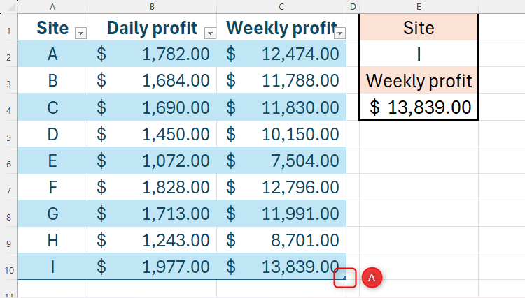
Second, if I were to add an extra row to my table by clicking and dragging the handle in the bottom-right corner (labeled “A” in the screenshot below), and then fill the extra row with additional data, the structured references I’ve already used in my spreadsheet would apply automatically to this new data.
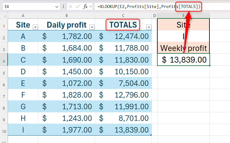
In this example, I’ve added data for an extra site (row 10). Not only did the weekly profit calculate automatically when I added the daily profit, but I also changed the site reference in cell E2 to site I, and the data has been retrieved correctly. If I had used direct references, I would have had to make several manual adjustments to achieve the same outcome.
Third, if I were to add another column between my “Daily profit” and “Weekly profit” columns, I could rest assured in the knowledge that any references to my existing columns would remain secure, as I’ve referenced the column names rather than the letter associated with each column.
Finally, structured references are dynamic. If I change the name of one of my table columns, all related structured references will update accordingly. In this example, I’ve changed my “Weekly profit” column to “TOTALS,” and the XLOOKUP formula in cell E4 has adopted this amendment.
In short, as soon as you create a table in Excel, you should be thinking about using structured references to make the most of your data.
Alongside the benefits listed above, structured references also use less of your computer’s memory than direct references—just one of the many ways to speed up your Excel spreadsheets.


