As a long-term Excel enthusiast, I have always enjoyed using VLOOKUP, one of Excel’s best-known lookup functions. However, Microsoft’s introduction of XLOOKUP in 2019 changed everything. Once I realized how useful XLOOKUP is, I knew I’d never look back.
I’ll use direct cell references to exemplify my points in this article, as they are clearer than structured references. I also won’t talk explicitly about HLOOKUP because—other than its direction—it works in exactly the same way as VLOOKUP.
The Syntaxes: XLOOKUP and VLOOKUP
Before I explain why I prefer XLOOKUP to VLOOKUP, I’ll show you how they work.
XLOOKUP
XLOOKUP has six arguments:
=XLOOKUP(a,b,c,d,e,f)
where
- a (required) is the lookup value,
- b (required) is the lookup array,
- c (required) is the return array,
- d (optional) is the text to return if the lookup value (a) is not found in the lookup array (b),
- e (optional) is the match mode, and
- f (optional) is the search mode.
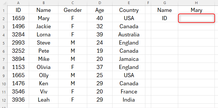
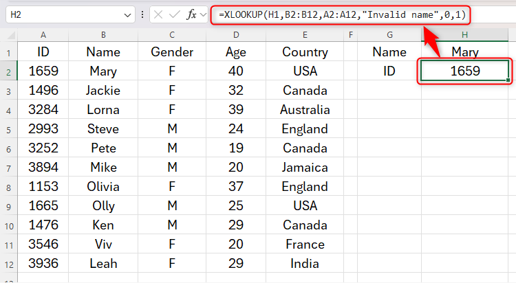
In this example, I want Excel to look up the employee ID based on the name in cell H1, and return the result to cell H2.
To do this, I will type the following formula into cell H2:
=XLOOKUP(H1,B2:B12,A2:A12,"Invalid name",0,1)
In this case, cell H1 contains the value Excel needs to look up (Mary), B2 to B12 is where that value can be found (employees’ names), A2 to A12 is where the corresponding result will be pulled from (employees’ IDs), and “Invalid name” is what I want Excel to return if the lookup value isn’t anywhere to be found in the lookup array.
I’ve gone for the default values for arguments e and f because I want an exact match, and I want Excel to search from the top of the lookup array (more on these later).
VLOOKUP
Here’s the VLOOKUP syntax, which has four arguments:
=VLOOKUP(a,b,c,d)
where
- a (required) is the lookup value,
- b (required) is the lookup and return array,
- c (required) is the column index number, and
- d (optional) is the match mode.
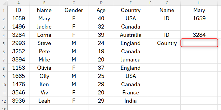
In this example, I want Excel to look up the nationality based on the employee ID in cell H4, and return the result to cell H5.
To do this, in cell H5, I will type
=VLOOKUP(H4,A2:E12,5,FALSE)
because cell H4 contains the lookup value (ID 3264), cells A2 to E12 are where Excel needs to find that value and the corresponding return, the fifth column (the country) is the array in which the result will be found, and I want an exact match (FALSE).
No Need to Count Columns
One key difference between VLOOKUP and XLOOKUP is that the former requires me to specify a column index number where the result will be found, whereas the latter doesn’t. This is because VLOOKUP combines the lookup and return arrays into one argument, whereas XLOOKUP defines them in two separate arguments.
VLOOKUP
Having to specify the column index number in VLOOKUP can lead to several issues:
- It’s easy to accidentally miscount the columns, especially if your lookup array is hundreds of columns across.
- Adding or removing columns could affect the accuracy of the column index number.
- The lookup array must be the leftmost column, and the return array must be to the right. This restricts VLOOKUP’s versatility.
XLOOKUP
On the other hand, XLOOKUP contains the lookup array as a separate argument, meaning you can appreciate the following benefits:
- There’s no counting involved! Simply use your mouse to select the return array when you get to that part of your formula. This saves time and aids accuracy.
- Because the return array is within a specified range of cells, removing or adding columns to your spreadsheet won’t affect your XLOOKUP formula.
- The return array can be on either side of the lookup array, meaning XLOOKUP is more versatile than VLOOKUP.
More Approximate Match Options
Both VLOOKUP and XLOOKUP can return an exact match (the exact corresponding value in a row) and an approximate match (a nearby corresponding value).
VLOOKUP
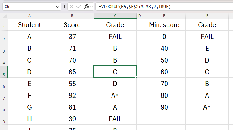
More specifically, VLOOKUP’s approximate match (indicated by TRUE in the formula) searches down the lookup array until it finds a value that’s larger than the lookup value. It then returns the value that is one row up from there.
Take Student D’s score of 65 in the example below. VLOOKUP takes the lookup value of 65, reviews the lookup array, finds the first value that’s larger than the lookup value (in this case, 70), and then returns the grade from the row above (grade C).
This presents two drawbacks. First, the lookup array must be listed in ascending order. Second, I have to add a FAIL row to the lookup array, as I don’t have the option in VLOOKUP to state a non-matching argument.
XLOOKUP
On the other hand, XLOOKUP offers three alternatives to VLOOKUP’s one-dimensional approximate match:
- -1: This returns the next smallest value in the lookup array if there’s no exact match.
- 1: This returns the next largest value in the lookup array if there’s no exact match.
- 2: This uses wildcards to allow for more flexible lookups.
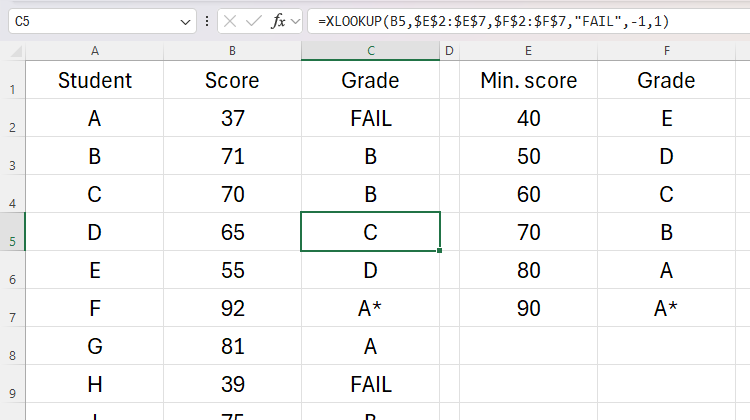
Again, take Student D as an example. With a score of 65, Excel will see that the next smallest value in the lookup array is 60, and the next largest value is 70. Since the student hasn’t yet reached the threshold for grade B (70), I need Excel to take the next smallest value in the lookup array (60) to return grade C from the return array. So, I will type -1 as the matching option in the formula.
This means that the lookup array doesn’t have to be in order—Excel scours the whole lookup array to find the nearest higher or lower values if there’s not an exact match. I can also omit the FAIL row from my lookup array because if a student’s score does not match any grades, I can use the fourth argument in the XLOOKUP syntax to return the word FAIL.
More Search Modes (Directions)
While VLOOKUP searches from first to last, returning the first matching value, XLOOKUP offers four search options.
VLOOKUP
In most lookup scenarios, searching the lookup array from first to last will return the results you need. For example, if you have a directory of phone numbers and people’s names, using VLOOKUP to find the phone number based on the name you input will work just fine, as that person’s name is only likely to appear once.
XLOOKUP
However, XLOOKUP lets you choose the search orientation:
- 1: Search first to last
- -1: Search last to first
- 2: Binary search (with the lookup array in ascending order)
- -2 Binary search (with the lookup array in descending order)
The benefit of a last-to-first lookup is that you can find the most recent occurrence of a value in a lookup array that is listed in date order. To achieve this with VLOOKUP, you would have to reverse the order of the data first.
Define the Error Output
A really useful feature of XLOOKUP is the “if not found argument,” which VLOOKUP doesn’t have.
VLOOKUP
If a value is not found in an exact match VLOOKUP formula, Excel returns the dreaded #N/A error message. To fix this, I’ve always embedded VLOOKUP functions within the IFERROR function so that I can define the output if VLOOKUP doesn’t find a match.
=IFERROR(VLOOKUP(B6,$E$2:$F$8,2,TRUE)," ")
While this is a reasonable solution, it makes formula writing much more complex and can hide issues that might affect the accuracy of your data analysis.
XLOOKUP
Since XLOOKUP comes ready-made with an “if not found” argument, you can define what happens if the value does not appear in the lookup, saving you from having to embed the formula within IFERROR.
Return a Spilled Array
One of VLOOKUP’s most stubborn properties is that it can only return a single match, whereas XLOOKUP can return a range.
XLOOKUP
In this example, typing
=XLOOKUP(I1,A2:A7,B2:F7)
looks up the value in cell I1 (in this case, Quizpicable Me), looks for that value in cells A2 to A7, and returns all the corresponding values as a spilled array.
VLOOKUP
If I were to try to replicate this using VLOOKUP, I would type
=VLOOKUP(I1,A2:F7,2:6)
but this returns a #REF! error because the third argument (column index number) can only be a single digit, not a range. This means that XLOOKUP is much more adaptable, as it can return either a single value or a range, depending on the parameters you add to the formula.
Since pre-2019 versions of Excel don’t support XLOOKUP, don’t discard VLOOKUP and HLOOKUP altogether! There may still be cases when you need to use them, like if you’re sending a spreadsheet to someone who hasn’t upgraded their Office package for a few years.


