Once, if you wanted to add checkboxes to your Excel spreadsheet, you had to use Form Controls in the Developer tab, a route that required some level of expertise. However, in June 2024, Microsoft introduced a much simpler way to use checkboxes.
How to Add and Remove Checkboxes
Excel’s Checkbox option is in the Controls group of the Insert tab on the ribbon. By default, the Controls group isn’t immediately visible when you open the Insert tab, so first, you’ll need to enable it first.
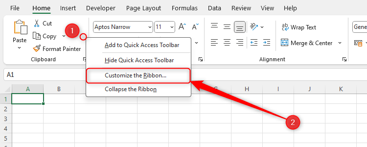
Right-click anywhere on the ribbon, and click “Customize The Ribbon.”
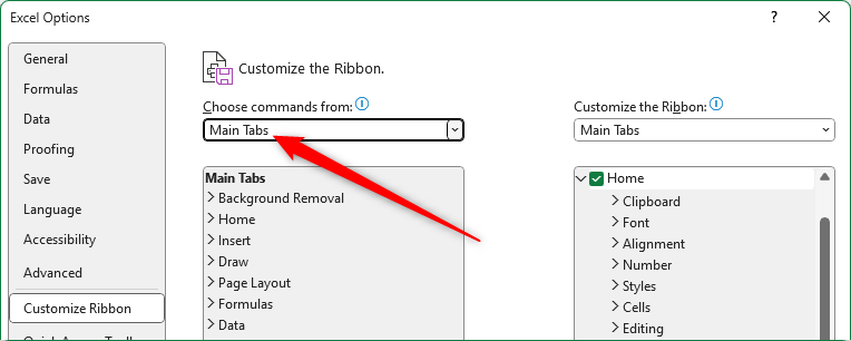
Now, in the Choose Commands From field, click “Main Tabs.”
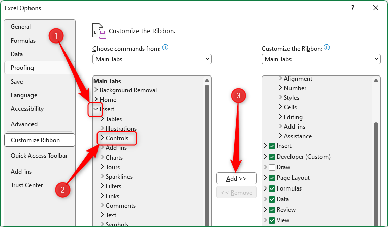
Next, click the “Insert” arrow to expand the Insert options, and select “Controls.” Then, to add this to the ribbon, click “Add.”
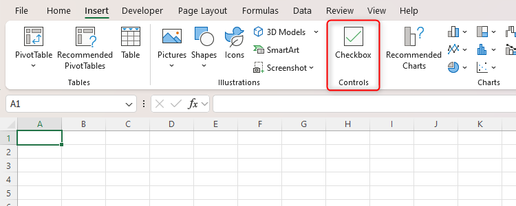
Finally, click “OK” to close the dialog box. You will then see Checkbox in the Controls group of the Insert tab on the ribbon, which you can click anytime to add one to your sheet.
To reposition the Checkbox button within the Insert tab on the ribbon, use the arrows on the right-hand side of the Customize The Ribbon dialog box.
What the Spacebar and Delete Keys Do to Checkboxes
Before you get to know the different ways you can use checkboxes, it’s worth knowing how they’re affected by different keys.
When you click the Checkbox icon in the Insert tab, you’ll see an unchecked checkbox added to whichever cell was selected. If you select more than one cell, several checkboxes will be added—one in each cell. While using your mouse to click the checkbox will add and remove the checkmark, you can also use the Spacebar to do the same, a handy tip if you prefer to work in Excel using only your keyboard. Likewise, if you select several cells containing a checkbox and press the Spacebar, they’ll all be checked and unchecked at the same time.
To delete a checkbox from your sheet, select the cell where the checkbox is located, and press Delete. If your checkbox is checked, pressing Delete will first uncheck the checkbox, and pressing it again will remove the checkbox altogether.
How to Use Checkboxes With IF
The first step in getting used to using checkboxes with Excel’s functions is to try it with the IF function alone.
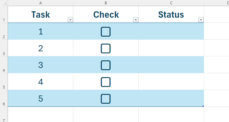
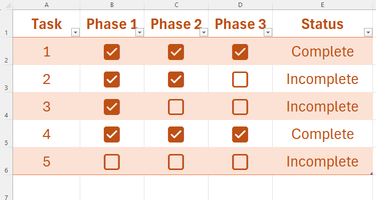
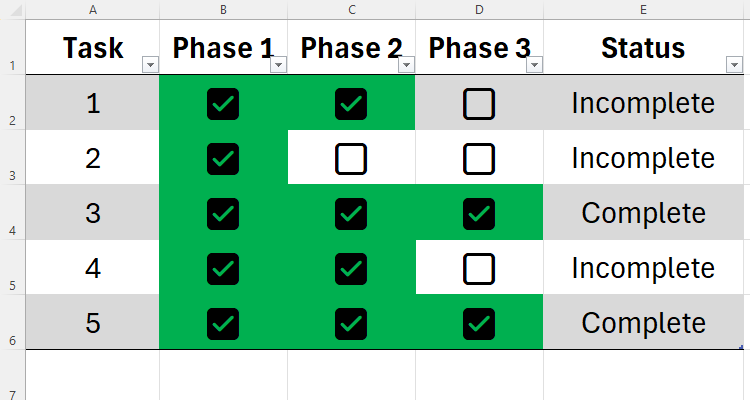
In the table below, we want the “Status” column to tell us whether the task is complete or incomplete based on whether the checkboxes are checked or unchecked.
When a checkbox is checked, it has a value of TRUE, and when unchecked, it’s FALSE. So, when using the IF function, these are the arguments that we will tell Excel to consider.
Starting in cell C2, we will create an IF formula with the following syntax:
=IF(x=y,"a","b")
where x is the cell containing the checkbox, y is TRUE or FALSE, a is the result we want to produce if the condition we entered is fulfilled, and b is the result if the condition isn’t fulfilled.
In our case, we’ll type
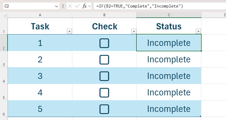
=IF(B2=TRUE,"Complete","Incomplete")
because we want Excel to find out whether the checkbox in B2 is checked, and produce the words “Complete” or “Incomplete” accordingly in C2.
Remember to use quotation marks around values
a
and
b
if you want Excel to produce text based on the checkbox’s status.
If you have formatted your table using Excel’s table formatter, when you press Enter after typing the above formula, you’ll see the formula automatically duplicated to the other cells in that column.
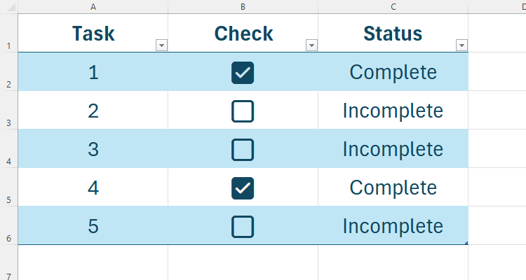
Now, check some of the checkboxes to see the outcomes in column C change.
If you click and drag the table handle (in the bottom-right corner of the formatted table) downwards, the new row will automatically contain the checkbox and the status formula you added.
How to Use Checkboxes With AND or OR
We’re now ready to use the checkboxes to check the progress of tasks containing more than one stage.
Using Checkboxes With AND
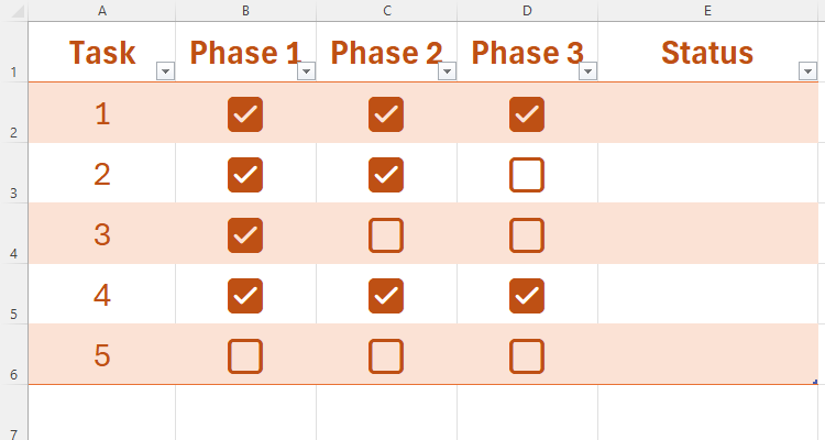
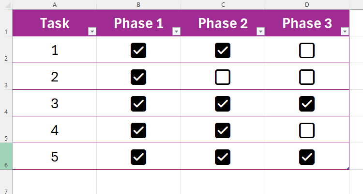
In this example, we want the “Status” column to tell us whether all phases of each task have been checked.
This is why we need to use the AND function alongside the IF function—the AND tells Excel we’re evaluating several criteria at the same time.
Here’s the syntax:
=IF(AND(x:y=z)"a","b")
where x:y is the range containing the checkboxes, z is TRUE or FALSE, and a and b are the results we want to see, depending on whether all the conditions are met.
So, in our case, we’ll type
=IF(AND(B2:D2=TRUE),"Complete","Incomplete")
because we want Excel to evaluate the checkboxes in cells B2, C2, and D2, telling us whether or not they’re all checked.
Using Checkboxes With OR
You can also follow the same principle with the OR function:
=IF(OR(x:y=z)"a","b")
where x:y is the range containing the checkboxes, z is TRUE or FALSE, and a and b are the results we want to see. This tells Excel to evaluate the checkboxes to see if any (rather than all) are checked.
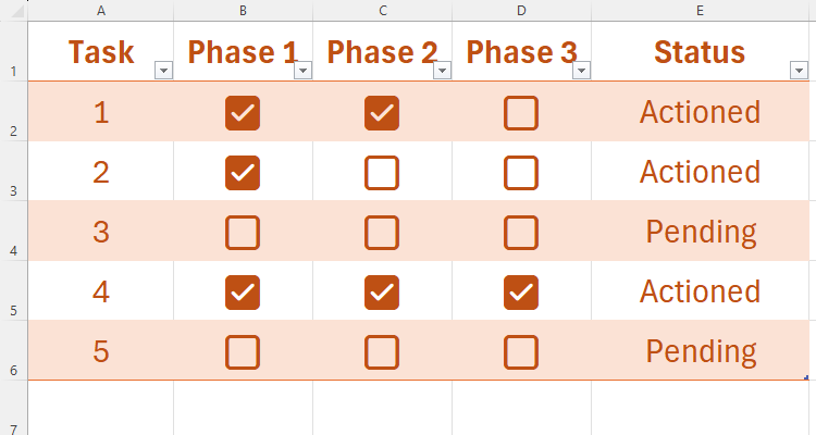
In this example, Excel tells us whether a task is pending (if none of the checkboxes are checked) or actioned (if any of the checkboxes are checked), as we have typed the following formula:
=IF(OR(B2:D2=TRUE),"Actioned","Pending")
How to Apply Conditional Formatting on Checkboxes
To make it even easier to visualize your data and track task progress, you can use Conditional Formatting to apply colors to the checkboxes or the cells where they’re located.
In this example, we want the cells containing the checkboxes to turn green when they’re checked.
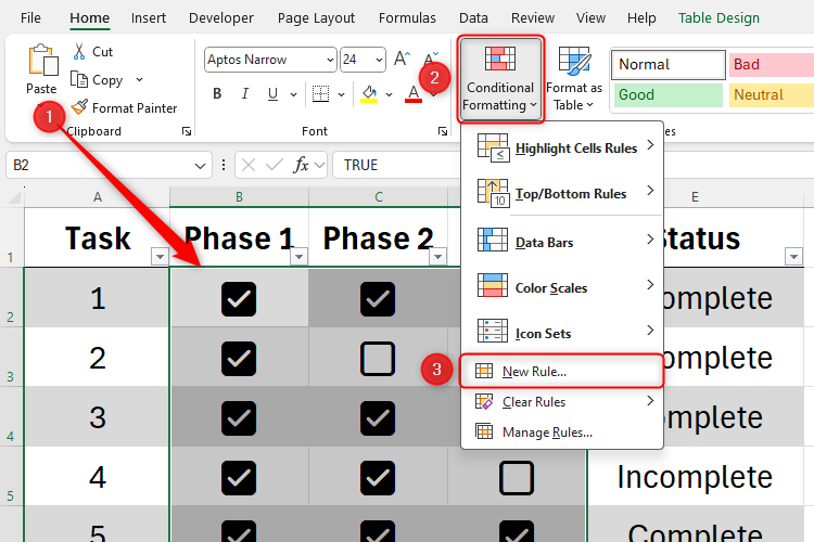
To do this, we need to select all the cells containing the checkboxes, click “Conditional Formatting” in the Home tab, and choose “New Rule.”
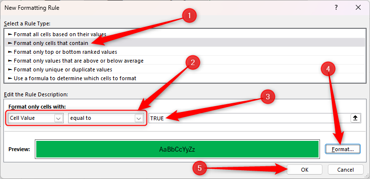
In the New Formatting Rule dialog box, follow these steps:
- Click “Format Only Cells That Contain.”
- Set the first and second drop-downs as “Cell Value” and “Equal To,” respectively.
- Type TRUE or FALSE, depending on whether you want the formatting to apply to a checked or an unchecked box.
- Click “Format,” and set the formatting according to what you want to happen when the checkboxes are checked or unchecked. In our case, we’re formatting the cells to be filled with green when the checkboxes are checked.
- Click “OK.”
How to Apply Conditional Formatting in Other Cells Based on the Checkboxes
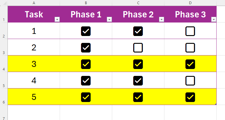
The final option is to format the whole row if all its checkboxes are checked. In our case, we want to clearly show that tasks 3 and 5 are complete.
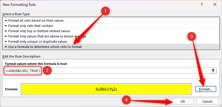
Start by selecting the entire table (except for the header row), and launch the New Formatting Rule dialog box by clicking Conditional Formatting > New Rule.
Then, use the following steps:
- Click “Use A Formula To Determine Which Cells To Format.”
- In the empty field box, type =AND($B2:$D2,”TRUE”), where $B2:$D2 are the cells containing the checkbox on the first row of the table, and “TRUE” tells Excel to apply the formatting when all the checkboxes are checked. Make sure you add the dollar symbol before the column references ($B2 and $D2)—this tells Excel that we want to apply the Conditional Formatting rule to all rows within those fixed columns.
- Click “Formatting” to determine what happens when the condition you’ve set is met. In our case, we’re choosing a yellow fill.
- Click “OK.”
Checkboxes aren’t the only way to track your task progress. Indeed, you can create a whole dashboard of data in Excel to monitor your workflow at a glance.


