How to Use the GROUPBY Function in Excel

Excel’s GROUPBY function lets you group and aggregate data based on certain fields in your table of data. It also offers arguments that allow you to sort and filter your data, so you can tailor the output to meet your specific needs.

Although you can use pivot tables to achieve similar outcomes to the GROUPBY function, the GROUPBY function refreshes automatically if your data changes or is reordered, and it also lets you embed more functions for more refined data sorting.

The GROUPBY Syntax

The GROUPBY function has eight arguments:

=GROUPBY(a,b,c,d,e,f,g,h)

Arguments a to c are required:

• a (row fields): The range (one or more columns) containing the values or categories by which the data is to be grouped.
• b (values): The range (one or more columns) containing the values that aggregate the data.
• c (function): A function used to aggregate the values in argument b.

Arguments d to h are optional, and you can learn more about these in the final section of this article:

• d (field headers): A number that specifies whether you selected headers in arguments a and b, and whether they should be displayed in the output.
• e (total depth): A number that determines whether the output should display totals.
• f (sort order): A number that indicates how the result is ordered.
• g (filter array): An array-oriented formula that filters out unwanted information.
• h (field relationship): A number that specifies the field relationships when multiple columns are provided in argument a.

GROUPBY in Action: Using the Required Arguments Only

If you’re overwhelmed by the large number of arguments that the GROUPBY function has, it’s important to note at this stage that the GROUPBY function works perfectly well even if you only populate arguments a, b, and c. So, first, I’ll show you how the GROUPBY function works with these three arguments alone.

Let’s imagine you own a chain of restaurants that serve up different dishes from different cuisines, and you’ve totted up the total sales and average customer rating for each cuisine-dish combination.

While these figures are useful, maybe you’re more interested in how the data compares across different categories. Specifically, you might want to find out the total cash each cuisine brings in, and the average customer rating for each type of dish.

Because the GROUPBY function returns spilled arrays, you can’t use formatted Excel tables for their results.

Let me take a moment to explain why GROUPBY would be my function of choice for executing these tasks for this specific dataset. If each cuisine and each dish only appeared once in the table, you would simply use the filter buttons to reorder and analyze your data. However, since cuisines and dishes are repeated, using the GROUPBY function will let you pull data from within common categories together, giving you a clearer whole-picture idea of the sales and rating distributions.

To find out the sales totals for each cuisine, in cell F2, type:

=GROUPBY(

Since you’re looking to group the data by cuisine, select the cells containing this variable, and add a comma. In this case, because the data is in a formatted Excel table called TabFood, a structured reference to the column name is added to my formula:

=GROUPBY(TabFood[Cuisine],

​​​​

Then, since you’re looking to see the total sales for each of those cuisines, select the cells containing these figures, and add another comma:

=GROUPBY(TabFood[Cuisine],TabFood[Sales],

The final mandatory argument is the function to be used on the aggregating data. In this case, since you want to find out the total sales for each cuisine, you need to insert the SUM function, and close the parentheses:

=GROUPBY(TabFood[Cuisine],TabFood[Sales],SUM)

As well as using straightforward functions like SUM and AVERAGE in argument c, you can also use Excel’s LAMBDA tool to create a function tailored to your needs.

When you press Enter, you’ll see that Excel has aggregated the total sales for each cuisine. Since you haven’t included any of the optional arguments in the GROUPBY function, the data is sorted in alphabetical order according to the values in column F by default, and there’s a total row at the bottom of your extracted data.

As the values in column G are financial, select the data and click the “Accounting” icon in the Number group of the Home tab on the ribbon.

Now, you want to find out the average customer rating for each type of dish, and the process for doing so is very similar.

In cell I2, type:

=GROUPBY(

Next, select the cells containing the category by which you want to group the data. In this case, it’s the different dishes. Remember to add a comma after each argument to move to the next.

=GROUPBY(TabFood[Dish],

Now, select the cells containing the data to be aggregated, and add another comma:

=GROUPBY(TabFood[Dish],TabFood[Customer rating]

Finally, because your aim on this occasion is to find out the average customer rating for each dish type, the function argument needs to be AVERAGE.

=GROUPBY(TabFood[Dish],TabFood[Customer rating],AVERAGE)

After you press Enter, Excel will average the customer ratings for each dish type. Again, in the absence of any optional arguments, the data is sorted in alphabetical order according to the values in the left-hand column by default, and there’s a handy total row at the bottom.

As the values in column J are decimalized averages, tidy up the number of decimal places on display by clicking the “Increase Decimal” and “Decrease Decimal” buttons in the Number group of the Home tab.

If you’re happy with your GROUPBY result at this stage, you can stop reading here. However, continue reading to learn about GROUPBY’s optional arguments.

GROUPBY in Action: Using the Optional Arguments

Even though the GROUPBY function having five optional arguments alongside the three required arguments makes it seem more complicated, these additional options are actually only there to help you create an output that is more tailored to your needs. What’s more, you can choose which optional arguments you want to use and skip over the ones you don’t.

Below, I’ll cover each of the optional arguments, so you can see how they will affect your data when you choose to include them.

Use a comma to jump from one argument to the next. For example, if you want to include the fourth and sixth arguments, but not the fifth, type [fourth argument],,[sixth argument]. The fifth argument would have been between where the two commas are positioned, but since there’s nothing in that space, Excel knows you’ve deliberately left this argument blank.

In the examples I used above, I typed the output column headers manually, since they’re not included in the result by default. However, if you want your output data to include the column headers as well as the data they contain, use the field headers argument.

Start by typing your GROUPBY formula, including the first three (required) arguments. In this case, let’s assume you want to group the cuisines by average customer ratings:

=GROUPBY(A1:A21,D1:D21,AVERAGE

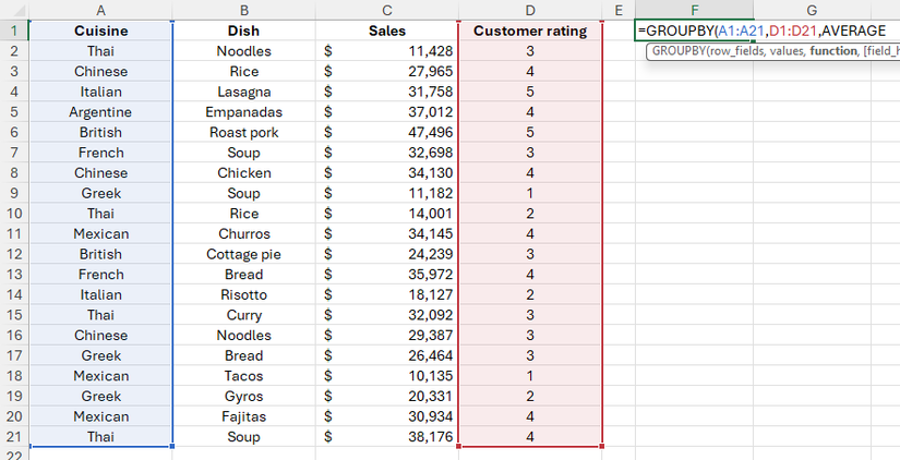
Notice how the header rows are included within the selections. Indeed, when selecting your data for the first two arguments, you should think ahead about whether you want your output data to duplicate the headings in your table.

Row fields and values arguments must be the same size. If you select headers in one, you must select headers in the other.

Finally, type a comma to move to the field headers argument and type:

• 1 if you have selected the headings in the first two arguments, but you don’t want them to show in the result,
• 2 if you haven’t selected headings in the first two arguments, but you want Excel to generate generic headings in the result, or
• 3 if you have selected the headings in the first two arguments, and you want Excel to show them in the result.

Here’s the result when I type:

=GROUPBY(A1:A21,D1:D21,AVERAGE,3)

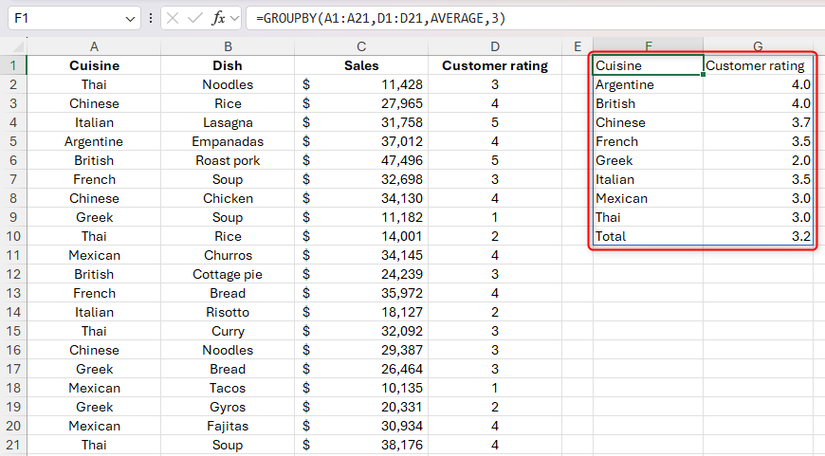
I can now format my duplicated column headings so that they’re clearly distinguishable from the data, just like in the original table.

Total Depth

The total depth argument lets you decide whether you want the result to display grand totals and, if you do, whether they should sit at the top or the bottom of your data. This argument also lets you choose whether to show subtotals.

For the total depth argument, type:

• 0 if you don’t want any totals or subtotals to be displayed,
• 1 if you want only the grand total to be displayed at the bottom of the result,
• 2 if you want subtotals to appear at the bottom of each result category, and a grand total at the bottom of the overall result,
• -1 if you want only the grand total to be displayed at the top of the result, or
• -2 if you want subtotals to appear at the top of each result category, and a grand total at the top of the overall result.

The options to display subtotals (2 and -2) only work if the row fields argument contains more than one column of data (in other words, subfields).

In this example, I’ve typed:

=GROUPBY(A1:B21,C1:C21,SUM,,2)

​​​​​​which uses commas to skip over the field categories argument, and tells Excel that I want subtotals to appear beneath each category and a grand total at the bottom of the data. I’ve then applied direct formatting to the subtotal rows to make the data easier to read.

Sort Order

The sort order field lets you tell Excel whether and how you want to sort the result. Using this argument really highlights why the GROUPBY function can be more useful than using a pivot table: as soon as you change any data in your original table, the whole output data reorders according to the sort order argument, whereas pivot tables require a manual refresh.

The number you enter for this argument represents the column in the result. For example, if you type 1, this will sort the result by the first column in ascending or alphabetical order. On the other hand, typing -1 will sort the result by the first column in descending or reverse alphabetical order.

In this example, I’ve typed:

=GROUPBY(A1:A21,C1:C21,SUM,,,-2)

which sorts the second column (sales) in descending order.

Filter Array

The filter array argument is less likely than the previous optional arguments to be used, though it can come to the rescue if your original data table contains rows that could interrupt your data.

In this example, the years in cells A2, A8, and A17 interrupt the GROUPBY function’s result.

I can use the filter array argument to tell Excel to ignore any cells in column A that contain numbers through the ISNUMBER function:

=GROUPBY(A1:A24,C1:C24,SUM,,,,ISNUMBER(A1:A24)=FALSE)

Field Relationship

Finally, the field relationship argument controls how data is grouped when the row fields argument references more than one column.

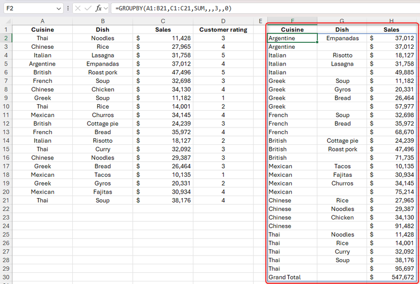
In this example, when the field relationship argument contains 0 (which is the default if the argument is omitted), GROUPBY returns a hierarchical result table, with each column individually represented with separate rows of data.

=GROUPBY(A1:B21,C1:C21,SUM,,,3,,0)

On the other hand, when the field relationship argument contains 1, GROUPBY returns a result table that ignores hierarchy and sorts each column independently. In other words, categories aren’t nested, which is why you also can’t include subtotals in the result when you choose this field relationship option.

=GROUPBY(A1:B21,C1:C21,SUM,,,3,,1)

---

As well as using SUM and AVERAGE in the GROUPBY function argument, you can use the PERENTOF function, which turns the data into percentages to show the proportion a subset makes up of a whole dataset.