You may be well-accustomed to using cell references in Excel, but did you know you could go one step further and create your own cell references? This is where the INDIRECT function comes in handy.
What Does the INDIRECT Function Do?
Excel’s INDIRECT function turns a text string into a reference. This function has several practical benefits:
- It allows you to create dynamic references. For example, you can change a reference to a cell within a formula without changing the formula itself.
- The INDIRECT function is a great way to create links between worksheets within a workbook.
- You can use information you already have in your spreadsheet to create a reference.
- The reference created using the INDIRECT function will stay the same, even if your sheet’s structure changes.
The INDIRECT Syntax
By default, references in Excel use the A1 reference style, which means that it refers to the column first, and then the row number. However, the INDIRECT function enables you to switch these around.
This inverted order is known as the R1C1 reference style, where the “R” refers to a row, and the “C” refers to a column. For this reason, the INDIRECT function contains two arguments. Here is the syntax:
=INDIRECT(x,y)
where x is the reference text, and y (optional) is the reference style.
More specifically, x (the reference text) can be an A1-style reference, an R1C1-style reference, a predefined name, or a cell reference. If x refers to another workbook, that second workbook must be open. It’s also worth noting that you cannot reference another workbook if you’re using Excel for the web.
y (the reference style) is an optional argument. If you choose not to include this argument, Excel will automatically use the default A1-style reference, though you can also type TRUE here to force Excel to use this reference style. Typing FALSE will tell Excel to use the R1C1 reference style.
In this article, I will use A1-style references to show you how the INDIRECT function works. Once you’ve grasped its concepts, you can experiment using R1C1-style references.
The outcome of the INDIRECT function is a reference.
Things to Bear in Mind Before Using the INDIRECT Function
There are a few things you should know before you start working with INDIRECT in your spreadsheet:
- This is a volatile function, meaning it’s constantly trying to update. Using this function in a large spreadsheet could result in it being sluggish or even dysfunctional.
- To make full use of the INDIRECT function, you would benefit from first knowing how to create named references in Excel.
- The ampersand (&) operator is a great way to create a text string that can be used as a reference.
How to Use the INDIRECT Function
So that you can get your head around how you can use INDIRECT in practise, let’s see how it works in its most basic form.
Basic Examples
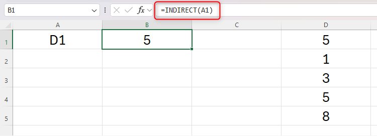
In this example, typing
=INDIRECT(A1)
into cell B2 turns cell A1 into a reference to cell D1. This is why the result is 5.
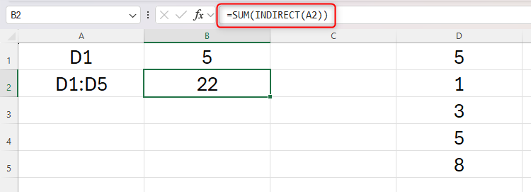
In this example, typing
=SUM(INDIRECT(A2))
into cell B2 first turns A2 into a cell reference, and then sums the cells in that reference. This is because the INDIRECT function is embedded within the SUM function.
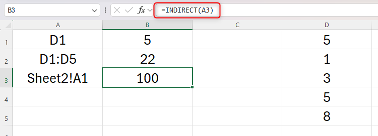
Now, let’s look at using the INDIRECT function to reference a cell in another sheet. Cell A1 of Sheet2 contains the number 100, and we want to create an INDIRECT reference to that cell in the current sheet. First, we need to type Sheet2!A1 into cell A3, and then we need to turn this into a reference using the INDIRECT function by typing
=INDIRECT(A3)
into cell B3.
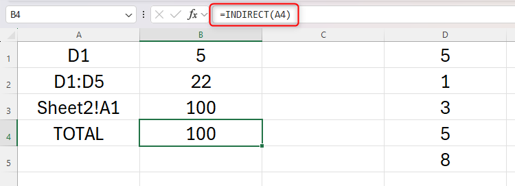
However, we can make this much easier by using a named reference. For example, if we were to rename cell A1 of Sheet2 TOTAL, we could use this within our INDIRECT reference. This is particularly handy if you’re creating a reference to another sheet, as it helps you avoid having to remember the exclamation point in the syntax. Also, if your sheet name changes, the INDIRECT reference will not adapt to this change, so using a named reference is a more secure and permanent alternative.
Real-world Example 1
Now that we understand how INDIRECT works, let’s explore how we can use it to make our worksheets tick in the real world.
As is often the case in Excel, there is more than one way to achieve the same outcome. For example, you could include
the TAKE function
to make the following process even more dynamic. However, our aim here is to exemplify the use of the INDIRECT function, so that you can then go ahead and use it in your own way.
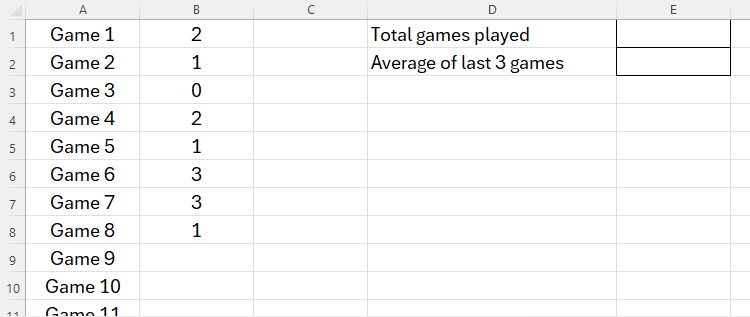
Here, we’re tracking the number of goals a football team scores in each game, and we want to work out the average for the previous three games.
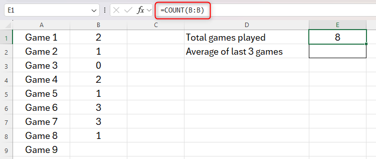
First, we will use the COUNT function to work out how many games the team has played so far. Typing
=COUNT(B:B)
into cell E1 will count the total number of cells in column B containing numbers, thus telling us how many games have been played.
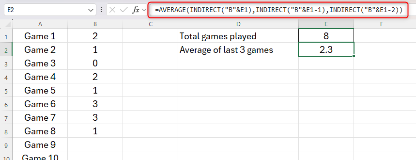
Now, we’re ready to use the INDIRECT function to turn the data in cell E1 into a reference. At this point, our aim is to find the average of the values in cells B6 to B8. Here’s how the INDIRECT function will help us to do this. Start by typing
=AVERAGE(INDIRECT
in cell E2, because we’re telling Excel that we ultimately want to find an average, and we’re also using the INDIRECT function to tell Excel where to look to calculate this average.
The first cell we will reference in our AVERAGE calculation is B8, so we will add
=AVERAGE(INDIRECT("B"&E1)
to our formula. Notice how we’ve used quotes around the column reference, as we’re using that text to create a cell reference.
The next cell we will reference in our AVERAGE calculation is B7, which is one cell upwards from B8. So, adding
=AVERAGE(INDIRECT("B"&E1),INDIRECT("B"&E1-1)
to our formula means that Excel will create a cell reference that starts in column B, and then minuses 1 from the value in E1.
Finally, we want to reference cell B6, which is two cells upwards from B8 in our AVERAGE calculation, and then add the closing parenthesis:
=AVERAGE(INDIRECT("B"&E1),INDIRECT("B"&E1-1),INDIRECT("B"&E1-2))
This correctly calculates the average of 3, 1, and 1, which is the total number of goals scored in the last three games.
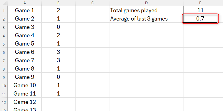
Now, when we add more data into column B, the value in cell E1 will increase, as the COUNT function recognizes that there are more values in column B, and the INDIRECT references will update accordingly to always capture the last three values in our AVERAGE formula. All this happens without having to change the formula we typed into cell E2.
Real-world Example 2
Let’s look at one more example. This time, we will use named references so that we can use INDIRECT with Excel’s VLOOKUP function.
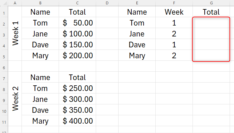
We want Excel to tell us how much money each of the four individuals made in either week 1 or week 2, with the option to change that week number if needed.
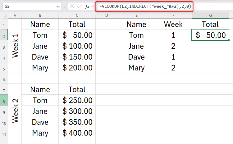
To begin, we need to name cells B1 to C5 as “week_1,” and cells B7 to B11 as “week_2.” Then, in cell G2, we will type
=VLOOKUP(E2,INDIRECT("week_"&F2),2,0)
because we want Excel to look up Tom’s value in the range we named “week_1,” and return the corresponding value in the second column of that range as an exact match.
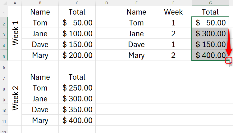
We can then use the fill handle to complete the data for the other three individuals, knowing that the references we created are both relative to their respective rows and also secure due to our use of named references.
Then, any changes to the values in columns C or F would automatically apply to the formula we have just written.
To complete the process of making your spreadsheet fully dynamic and tidy, you could add drop-down menus using Excel’s Data Validation tool. In the example above, you could have the individuals’ names accessible through a drop-down menu, so that the lookup table takes up only a single row.


