


Image used with permission by copyright holder
As you use Microsoft Excel more and more, you’ll find that the VLOOKUP function is a very popular tool for dealing with large Excel directories or databases. It allows the user to quickly find targeted information about a specific entry without needing to look through the entire spreadsheet.
Don’t worry, though — this function isn’t nearly as intimidating as it looks, and it can save a lot of time and allow for more freestyle analysis. Here’s how to use VLOOKUP in Excel.
Understanding the VLOOKUP pathing
The VLOOKUP function is divided into four different “arguments,” or values input into your function. These define exactly where VLOOKUP will pull information from, so while you start the function with the basic =VLOOKUP(), the four arguments that you put in those parentheses will be doing all the work.
In brief, you’ll be telling VLOOKUP the value you want to look up, the range where the value is located, the column where the return value is, and if the return needs to be exact or approximate. If you don’t have a lot of experience with Excel functions, that may not make much sense. Let’s make it easier by breaking each argument down into how it performs. Think of an example like an employee directory or a class grading sheet to see how this can work in real life.
Step 1: Select the first argument.
This is your lookup value, or the identifying information that you will use to pull data about one specific line in a database or directory. This is the space where you will be inputting information such as employee or class IDs, specific names, and so on. You can choose where this lookup value goes, but ideally, it will be close to the VLOOKUP for easy analysis and clearly labeled so you will always know what to input.
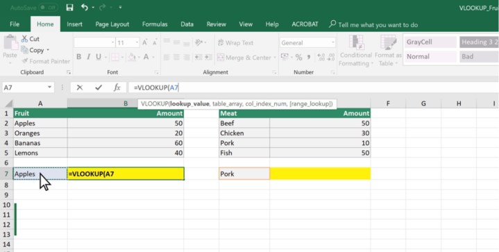
Image used with permission by copyright holder
Step 2: Select the second argument.
This is the range where your first argument, the lookup value, is located in the range. For example, if you are looking up a specific employee ID number, then this argument should contain the entire database. It’s simplest to manually click the very first entry and then drag your cursor all the way down to the final bottom-right entry at the end so it encompasses all the cells, holding all the values in the database. For very large databases, manually input the first entry (A2, for example), a colon, and the last entry (B5, in this case), like: A2:B5.
Note that the second argument should always start with the first (leftmost) column in the database or range. This is also why VLOOKUP won’t work well with horizontally oriented lists, but that’s rare in spreadsheets.
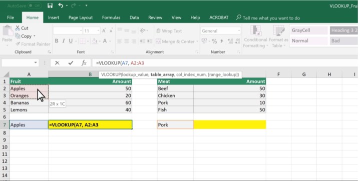
Image used with permission by copyright holder
Step 3: Select the third argument.
VLOOKUP now knows the full range of the database or table where it’s looking for information, but it needs a little more help. Now you need to select the column where the return value is located – aka the specific entry that you want when typing in your lookup value.
The third argument needs to be a number, not a column letter. Start counting from the first entry column on the list and count over to the right until you reach the column with the data that you’re interested in (like employee bonuses or student grades). Input this number into the function so that VLOOKUP knows what to return.
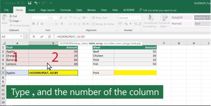
Image used with permission by copyright holder
Step 4: Select the fourth argument.
The fourth argument is a bit different: You can type FALSE or TRUE here to specify if you want to return either an exact match or an approximate match. You don’t have to do this step if you want to end the function here, but it does have its uses. A FALSE argument will return an error if it cannot find your input value – if, for example, the employee ID you enter doesn’t exist. A TRUE input will round to the closest possible result and return the desired value for that entry, which can simplify certain kinds of analysis.
With your VLOOKUP function complete, you can now start entering values in your lookup space and see the results that VLOOKUP returns.
Important notes to remember
-
VLOOKUP always paths to the right. It will not path left. Keep this in mind when arranging your lookup data.
-
Data ranges are disrupted when you add a new column in Excel, so again, consider this when making changes.
-
VLOOKUP doesn’t understand duplicates. For example, if two employees have the same last name, VLOOKUP will simply stop at the first one on the list, regardless if it’s the name you wanted or not. That’s why the function is often used with full names or ID numbers instead.
-
VLOOKUP is case sensitive, so it can tell the difference between looking up a capitalized word and one that isn’t.
-
Like other Excel functions, it’s easy to expand VLOOKUP into a full table to return multiple values at once, depending on your project. Once you’re comfortable with the process, you can start using it in more complex ways!
Microsoft Excel affords considerable control over the data your store in it. VLOOKUP is a great way to find and return data, which can then be presented in various other ways. You probably know how to create a graph in Excel, but do you know how to create a pivot table?


