How You Can Use Wildcards in Microsoft Excel to Refine Your Search

Wildcards in Microsoft Excel let you search for partial matches, broaden your filters, and create formulas that reference cells containing certain strings. They represent non-specified characters to help you locate text values with “fuzzy” matches.

The Wildcards: Asterisk (*) and Question Mark (?)

There are two wildcards in Excel, and knowing their purpose is crucial to understanding how wildcards work overall.

The Asterisk Wildcard: Any Number of Characters

The first of the two wildcards in Microsoft Excel is an asterisk, which represents any number of characters, including no characters.

For example:

• *OK* matches with any cells that contain “OK,” with any number of characters before or after (including no characters).
• OK* matches with any cells that start with “OK,” with any number of characters (including no characters) after, but nothing before.
• *OK matches with any cells that end with “OK,” with any number of characters (including no characters) before.

The Question Mark Wildcard: Any Single Character

Microsoft Excel’s second wildcard is the question mark, which substitutes any single character.

For example:

• ?OK? matches with any cells that contain a single character before “OK,” and a single character after.
• OK? matches with any cells that contain a single character after “OK”, but nothing before.
• ?OK matches with any cells that contain a single character before “OK”, but nothing after.

Question Mark and Asterisk Wildcards Combined

You can also use the question mark and asterisk together to find results that have finite numbers of characters in some positions, but any number of characters in others.

For example,

• ??OK* matches with any cells that begin with two characters, then contain “OK,” with any number of characters at the end (including none).
• *OK? matches with any cells that begin with any number of characters (including none), then contain “OK,” and end with one more character.
• ?OK* matches with any cells that begin with a single character, then contain “OK,” and have any number of characters (including none) thereafter.

Canceling Wildcards: Tilde (~)

Sometimes, you might actually want to search for question marks and asterisks as characters in their own right in your Excel worksheet. This is where the third wildcard character—the tilde—comes into play: simply place it before the question mark or asterisk to tell Excel you don’t want them to be treated as wildcards.

For example:

• *~? matches with any cells that contain any number of characters (including none) at the start, and a question mark at the end.
• *~?* matches with any cells that contain any number of characters (including none) on either side of a question mark.
• *~*? matches with any cells that start with any number of characters, followed by an asterisk, followed by a single character.

Using Wildcards in Searches

One of the most common uses of wildcards in Microsoft Excel is to find characters in a workbook and, if needed, replace them with alternatives.

Find Character Strings

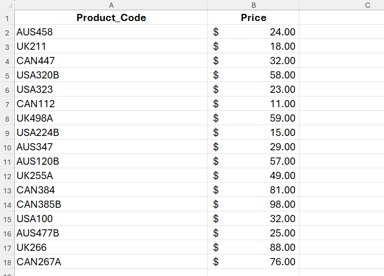
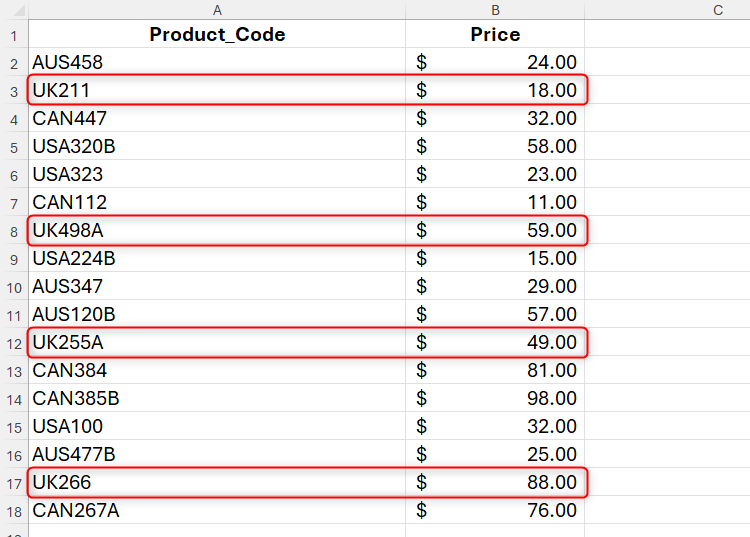
In this list of product codes, the letters at the beginning represent where the product was manufactured (AUS for Australia, UK for the United Kingdom, USA for the United States, and CAN for Canada), the first digit represents the relevant store department (1 is clothing, 2 is homeware, 3 is sports, and 4 is garden), and codes with a letter at the end are national sale only (A) or international sale only (B).

Let’s say you want to find all the homeware products that are for national sale only.

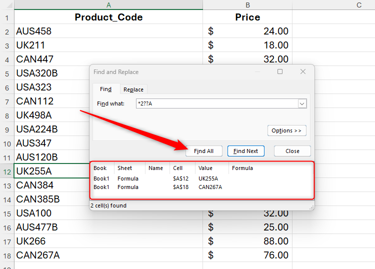
Press Ctrl+F to launch the Find tab of the Find And Replace dialog box, and in the Find What field, type:

*2??A

where

• The asterisk and the number 2 tell Excel to search for cells that start with any number of characters, followed by the number 2. You need to use an asterisk here, since some countries are represented by two letters while others are represented by three.
• The two question marks followed by the letter A tell Excel that the rest of the string must be made up of two characters and the letter A.

Then, when you click “Find All,” you’ll see a list at the bottom of the Find And Replace dialog box that shows any results that match these criteria.

Click any of the results in the Find And Replace dialog box to jump to the corresponding cell in your spreadsheet.

Now, let’s say your aim is to return the codes for all clothing products that aren’t restricted to national or international sales only (in other words, codes that contain a country and a three-digit number starting with 1, but don’t end with a letter).

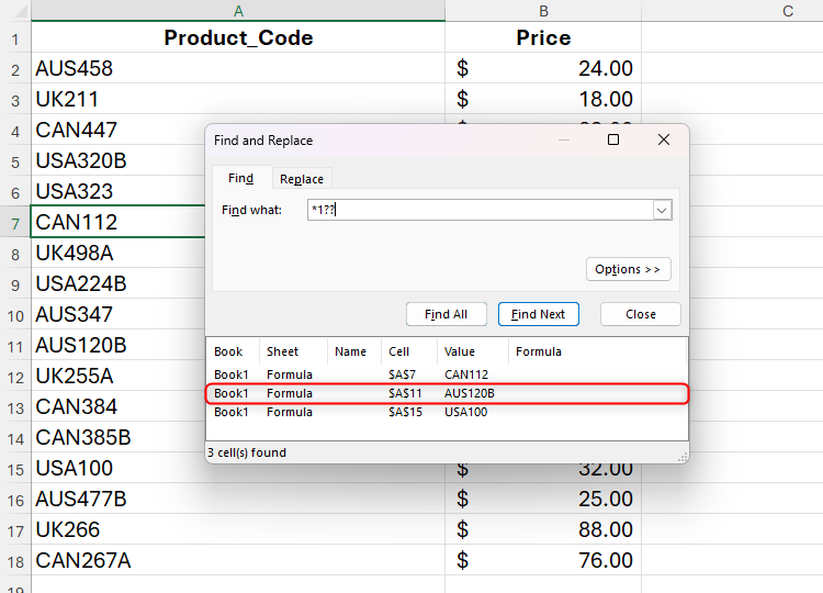
In the Find What field, type:

*1??

However, when you click “Find All,” a product ending in a letter shows up in the result, suggesting there’s something missing from the criteria.

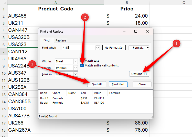
In fact, this happened because part of the erroneous code contains the substring you entered for the query. So, to exclude these and return only the codes that fully match your query, click “Options,” check “Match Entire Cell Contents,” and click “Find All” again.

This time, only the desired results are displayed.

Find And Replace Character Strings

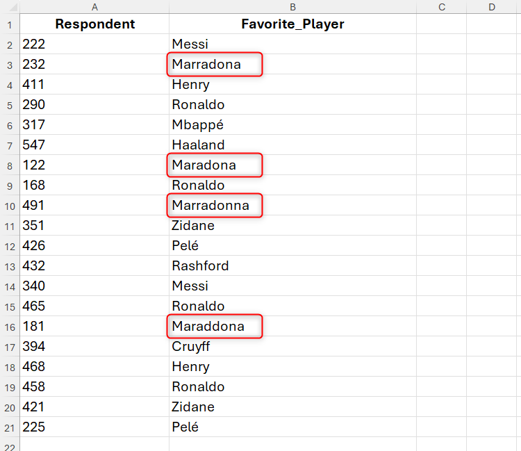
This Excel list shows respondents’ all-time favorite soccer players. However, Maradona’s name has been spelled in three different ways, and you want to amend the incorrect ones.

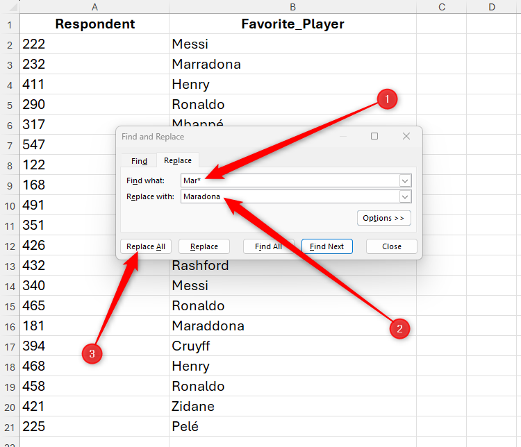
First, press Ctrl+H to launch the Replace tab of the Find And Replace dialog box. Then, in the Find What field, type:

Mar*

since all incorrect spellings start with these three letters, and it’s the only name in the list that starts with this character string.

Then, in the Replace With, type the correct spelling:

Maradona

and click “Replace All” to confirm the corrections.

Now, all cases of this player’s name are spelled correctly and consistently.

Using Wildcards in Formulas

As well as using wildcards in Excel’s Find And Replace dialog box, you can use them in arguments for various functions, such as XLOOKUP to generate a partial match lookup, COUNTIFS to count the number of cells that match multiple criteria, and many more.

In this example, you want to use the SUMIF function to work out the total price of products originating in the UK.

One way to do this would be to type:

=SUMIF(A2:A18,"UK*",B2:B18)

into a blank cell, where

• SUMIF adds values together based on set criteria,
• A2:A18 is the range containing the values to be tested,
• “UK*” tells Excel to find any cells in A2 to A18 starting with “UK,” followed by any number of characters, and
• B2:B18 is the array to sum.

Wildcards and text values must always be placed in quotation marks in Excel formulas.

However, suppose you then want to find the total price of products from another country. In the example above, you would need to change the formula manually, a method that takes time and is more likely to result in error.

Instead, type the criteria (in this case, “UK”) in a separate cell. Then, reference that cell in the formula, using the ampersand (&) symbol to separate the cell reference from the wildcard embedded in quotation marks:

=SUMIF(A2:A18,D2&"*",B2:B18)

Now, when you change the country code, the total updates.

Using Wildcards in Filters

Another use of wildcards in Microsoft Excel is in filters.

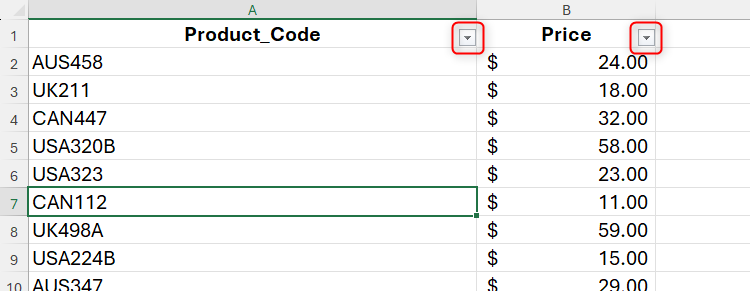
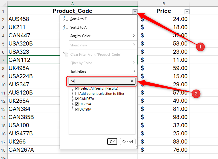
Whether you’re working in a formatted Excel table or an unformatted range, select any cell in the array, and press Ctrl+Shift+L to add filter buttons.

Now, let’s say you want to filter the product codes to include only those that contain the letter A at the end.

To do this, click the Product_Code filter button, and in the Search field, type:

*A

to include all codes ending in the letter A. Since the asterisk wildcard is placed before the letter A in the search, it doesn’t pick up any product codes containing A at the start (such as AUS458) or in the middle (such as USA320B).

Once you’ve previewed the results in the filter pop-up window, click “OK,” and see your data refined to match your criteria.

Points to Note

Before you go ahead and make use of wildcards in your Excel spreadsheet, take a moment to read these final pointers:

• When using wildcards in formulas, you’ll hit a hurdle if you try to find a digit in a range of numbers. This is because wildcards automatically convert numbers to text. However, searching for digits in a range of numbers using Excel’s Find And Replace tool or filters will work just fine, as will finding numbers in cells that also contain text values.
• Although many functions support the use of wildcards, some—including the IF function—don’t.
• Adding wildcards to formulas makes them more complicated, potentially increasing the risk of errors if you don’t take extra care. Always remember to embed wildcards within quotation marks in formulas!

---

As well as using wildcards to broaden your search capabilities in Excel, you can also use them to find and replace text in Microsoft Word. The major difference between the two is that, alongside the asterisk and question mark, Word also lets you use square brackets ([ ]) as wildcards to match more than one item.