For many years, I used the SUBTOTAL function in Microsoft Excel to create easily visible subtotals at the top of my worksheets. However, when I encountered AGGREGATE, this became my go-to function for achieving the same result but with more flexibility.
Before I explain further, let’s remind ourselves how the SUBTOTAL function works.
The SUBTOTAL Function
Microsoft Excel’s SUBTOTAL function is quite simple to use. It lets you perform subtotal calculations for ranges of cells, and you can decide whether you want to include manually hidden rows in the result.

Related
How to Use the SUBTOTAL Function in Microsoft Excel
See the subtotal of values with this simple Excel function.
However, rows that are filtered out are always excluded, and the SUBTOTAL function doesn’t work if there are errors in the data, unless you nest it within the IFERROR function. What’s more, SUBTOTAL only supports 11 functions, limiting its use if you want to perform more complex statistical calculations.
Here’s the syntax:
=SUBTOTAL(a,b,c)
where
- a (required) is a number that represents the function you want to use in the calculation,
- b (required) is the first range of cells to subtotal, and
- c (optional) represents the first of up to 252 more ranges to subtotal, each separated by a comma.
For argument a, 1 or 101 = AVERAGE, 2 or 102 = COUNT, 3 or 103 = COUNTA, 4 or 104 = MAX, 5 or 105 = MIN, 6 or 106 = PRODUCT, 7 or 107 = STDEV, 8 or 108 = STDEV.P, 9 or 109 = SUM, 10 or 110 = VAR, and 11 or 111 = VARP.
Numbers 1 to 11 for argument a force the result to include manually hidden rows, while 101 to 111 exclude manually hidden rows.
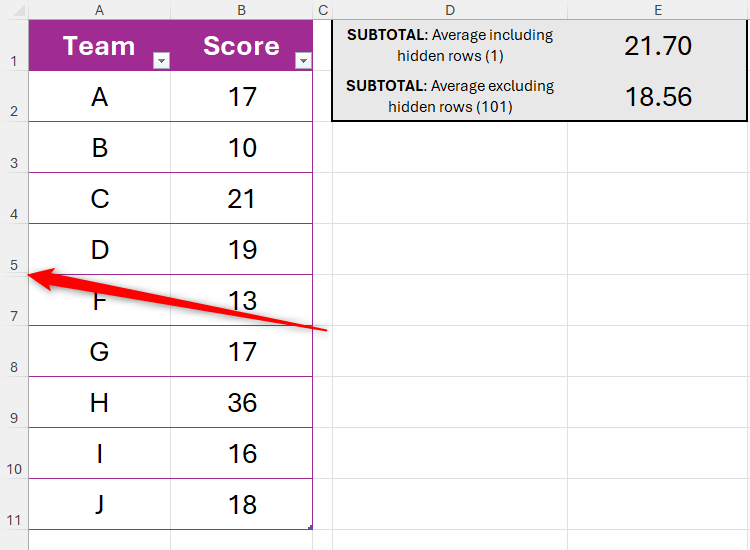
In this example, the SUBTOTAL function has been used to calculate the average of the values in column B, with row 6 (team E) hidden. The subtotal in cell E1 includes the hidden row (argument a = 1), while the subtotal in cell E2 doesn’t (argument a = 101).
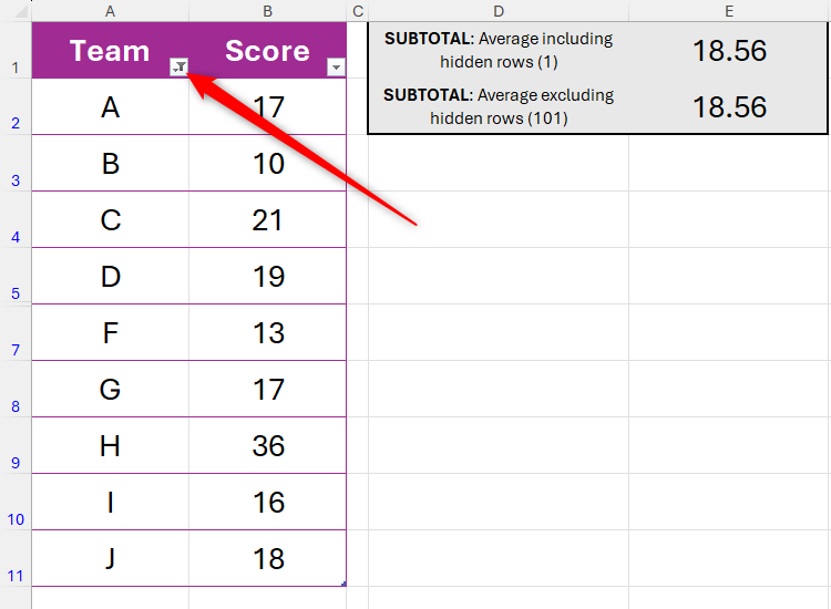
However, when the filter is used to hide the score of team E instead, both subtotals are the same, as there’s no way to get the SUBTOTAL to include filtered-out values.

Related
How to Sort and Filter Data in Excel
Microsoft Excel has power sorting and filtering options. Here’s how to use them in your spreadsheet.
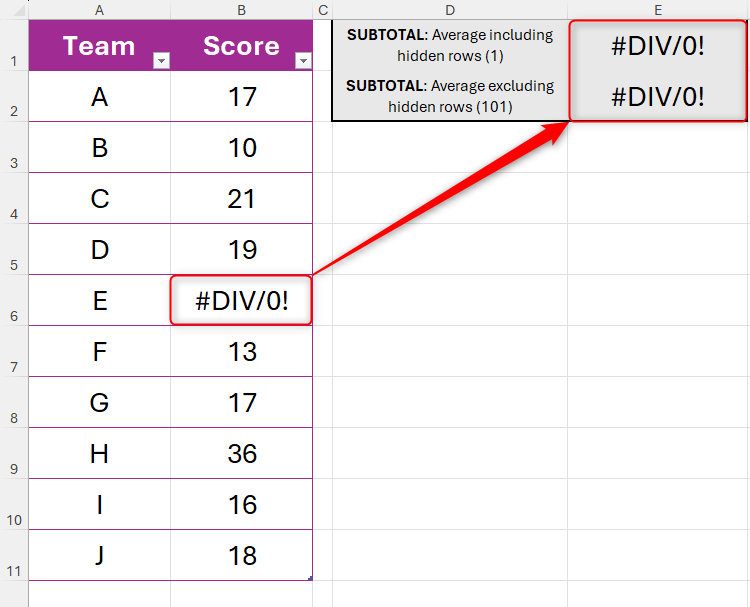
In this final example, you can see that the SUBTOTAL function returns an error if there’s an error in the range.
To avoid these issues, you can use the AGGREGATE function instead.
The AGGREGATE Function
The AGGREGATE function is similar to the SUBTOTAL function, but there are more options for the type of aggregation you want to create. Also, you have a wider choice of things you can exclude from the result, and you can make Excel ignore errors in your data.
In other words, compared to the SUBTOTAL function, AGGREGATE is more powerful and flexible.
The AGGREGATE function has two syntaxes—one for references and one for arrays—though you don’t need to worry about which one you’re using, as Excel selects the relevant one depending on the arguments you input.

Related
How to Use Excel’s AGGREGATE Function to Refine Calculations
Miss out hidden rows, errors, or nested functions in your formulas.
The syntax for the reference form of the AGGREGATE function is:
=AGGREGATE(a,b,c,d)
where
- a (required) is a number that represents the function you want to use in the calculation,
- b (required) is a number that defines what you want the calculation to ignore,
- c (required) is the range of cells on which the function will be applied, and
- d (optional) is the first of up to 252 additional arguments that specify further ranges.
If you’re working with arrays, the AGGREGATE function follows a slightly different syntax:
=AGGREGATE(a,b,c,d)
where
- a (required) is a number that represents the function you want to use in the calculation,
- b (required) is a number that defines what you want the calculation to ignore,
- c (required) is the array of values on which the function will be applied, and
- d is the second argument required by array functions like LARGE, SMALL, PERCENTILE.INC, and others.
The first difference to note between SUBTOTAL and AGGREGATE is that the latter has more options for argument a: 1 = AVERAGE, 2 = COUNT, 3 = COUNTA, 4 = MAX, 5 = MIN, 6 = PRODUCT, 7 = STDEV.S, 8 = STDEV.P, 9 = SUM, 10 = VAR.S, 11 = VAR.P, 12 = MEDIAN, 13 = MODE.SNGL, 14 = LARGE, 15 = SMALL, 16 = PERCENTILE.INC, 17 = QUARTILE.INC, 18 = PERCENTILE.EXC, and 19 = QUARTILE.EXC.
However, where AGGREGATE really trumps SUBTOTAL is in its ability to exclude certain values from the result (argument b):
|
Number |
What Is Ignored |
|---|---|
|
0 |
Nested SUBTOTAL and AGGREGATE functions |
|
1 |
Hidden rows, and nested SUBTOTAL and AGGREGATE functions |
|
2 |
Errors, and nested SUBTOTAL and AGGREGATE functions |
|
3 |
Hidden rows, error values, and nested SUBTOTAL and AGGREGATE functions |
|
4 |
Nothing |
|
5 |
Hidden rows only |
|
6 |
Errors only |
|
7 |
Hidden rows and errors |
So, let’s see it in action.
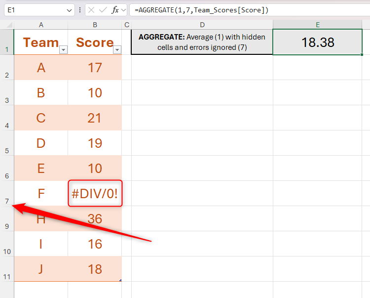
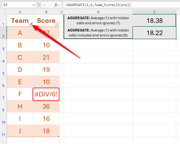
In this example, typing:
=AGGREGATE(1,7,Team_Scores[Score])
into cell E2 returns the average (argument a = 1) of the visible values in column B, ignoring the hidden value in row 8 and the error in row 7 (argument b = 7).

Related
How to Hide Cells, Rows, and Columns in Excel
There may be times when you want to hide information in certain cells or hide entire rows or columns in an Excel worksheet.
You wouldn’t be able to get the same result using the SUBTOTAL function alone in this scenario, as it can’t overlook errors without being nested within an IFERROR formula.
Even though bypassing errors is a good way to make your spreadsheet look tidier, don’t get into the habit of ignoring them altogether! They’re there for a reason and could help with troubleshooting.
On the other hand, typing:
=AGGREGATE(1,6,Team_Scores[Score])
into cell E3 returns the average (argument a = 1) of all the values in column B, including the value on row 8 that is filtered out and excluding the error (argument b = 6).
Once again, this wouldn’t be possible with SUBTOTAL, as it always includes filtered-out rows in the result, and there’s no way to bypass the error in the data.
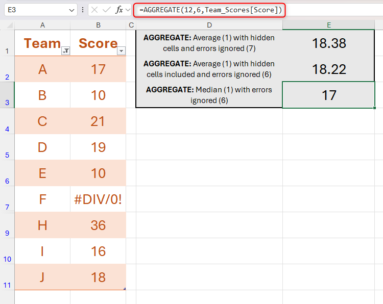
This time, in cell E3, the AGGREGATE function is used to generate the median (argument a = 12), one of the many calculations the SUBTOTAL function doesn’t allow:
=AGGREGATE(12,6,Team_Scores[Score])
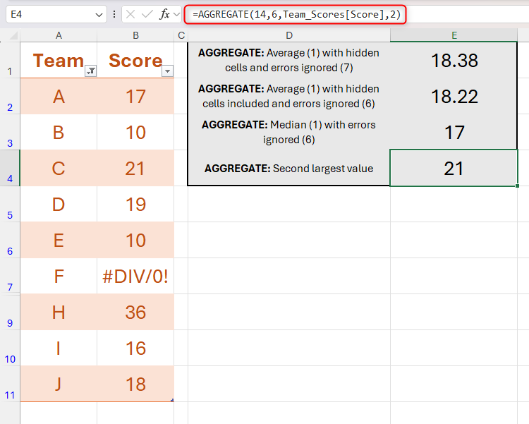
In a final example, argument d has been used to generate the second-largest value:
=AGGREGATE(14,6,Team_Scores[Score],2)
Summary: SUBTOTAL vs. AGGREGATE in Excel
Here’s a summary of Microsoft Excel’s SUBTOTAL and AGGREGATE functions:
|
Feature |
SUBTOTAL |
AGGREGATE |
|---|---|---|
|
Suitable for straightforward aggregations |
Y |
Y |
|
Suitable for complex statistical aggregations |
N |
Y |
|
Number of functions supported |
11 |
19 |
|
Can include or exclude manually hidden rows |
Y |
Y |
|
Can include or exclude filtered rows |
N |
Y |
|
Can ignore errors |
N |
Y |
|
Can ignore nested SUBTOTAL or AGGREGATE results |
Y |
Y |
|
Offers further options for array functions |
N |
Y |
Even if you think you’ve settled on a function that works for you, always double-check that there isn’t another function that does the job even better! Microsoft often introduces new functions that are upgrades from older ones—for example, I now use XLOOKUP instead of VLOOKUP, and XMATCH is much more user-friendly than MATCH.

